



A cloud-native, machine learning-optimized tile grid for land cover analysis
* This article is part of a Special Issue from FOSS4GNA.
1 Planet Labs PBC, San Francisco, CA, USA
TM: https://orcid.org/0009-0000-2192-1800
RCM: https://orcid.org/0009-0007-0482-1972
CBA: https://orcid.org/0000-0001-7392-4368
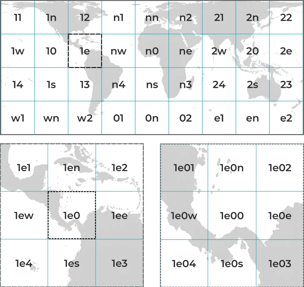
Abstract photo. A global tile grid with a hierarchical index built for multi-scale, area-based Earth observation analysis. Three views represent different levels of the tile hierarchy, centered globally (top), over Mesoamerica (lower left, dashed lines) and near the Isthmus of Panama (lower right, dotted lines).
Abstract
Geospatial tile partitioning underpins gridded Earth observation (EO) data processing, yet there is little consensus on how to define global tile grids for large-scale raster workflows. Existing tooling like Discrete Global Grid Systems and Tile Matrix Sets often prioritize geodesic or visualization properties, employing multi-region grids, non-rectangular extents, or quad-tree resolution hierarchies. These paradigms are not optimized for global, multi-scale satellite data, resulting in dataset fragmentation, computational overhead, and repeated resampling. To formalize a cloud-native grid optimized for machine learning and land cover analysis, this study evaluated six global map projections across four operational dimensions: total pixel footprint, geometric distortion, layout simplicity, and open source tooling compatibility. Additionally, the study assessed nonary tree grid layouts (3×3) in contrast to standard quad tree layouts (2×2). Following this analysis, we propose a novel grid specification with a 3×3 nonary tree layout that intrinsically aligns with common EO sensor scales, simplifying multi-scale analysis. The Lambert cylindrical equal-area projection (EASE Grid) was selected for its compact footprint and robust software support, conceding systematic angular distortions at high latitudes as a trade-off. A prefix-based tile encoding scheme is described that natively captures hierarchical depth and spatial relationships, streamlining metadata retrieval without complex spatial queries. Ultimately, this work presents a practical tile grid optimized for global EO workflows, illustrating a systematic approach to planetary-scale geoprocessing.
Keywords: Earth observations, geospatial analysis, global grid, machine learning, satellite data
Introduction
Large-scale satellite Earth observation (EO) data processing is a parallel computational problem (Stockinger et al., 2006, Afgan and Bangalore, 2008). Gridded raster data — Level 3 (L3) or Level 4 (L4) data products in particular (NASA, 2021) — can be partitioned into geospatial tiles and processed independently across distributed infrastructure. This paradigm underpins modern EO data cubes, planetary-scale processing platforms, and machine learning pipelines operating on satellite data. There is little agreement, however, on how global tile grids should be defined. Most global grids optimize for visualization or spatial partitioning, not for large-scale raster analytics. As a result, data products frequently adopt custom tiling schemes tailored to individual sensors or workflows (Brodzik et al., 2012, Bauer-Marschallinger et al., 2014, Lewis et al., 2017, Bauer-Marschallinger and Falkner, 2023). This fragmentation leads to recurring issues: resolution mismatches, repeated resampling, inconsistent tile naming, and computational overhead.
Several efforts have attempted to standardize spatial partitioning at a global scale. Discrete Global Grid Systems (DGGS), for example, subdivide the Earth into hierarchical cells—often hexagonal or otherwise non-rectangular—with well-defined indexing properties (Goodchild, 2000, Gibb et al., 2022). While these systems provide elegant solutions for spatial indexing and aggregation, they are typically not well-suited for raster-native processing. EO data are often represented with square pixels on regular grids, and transforming such data into non-rectangular or geodesic cell structures introduces additional reprojection, resampling, and computational costs. Another approach is to subdivide the land surface into regional projections to minimize local distortions, which was the approach of the Equi7Grid (Bauer-Marschallinger et al., 2014). They defined seven continental zones and assigned each its own equidistant projection. Managing multiple projections within a single grid is operationally complex, however, and encounters limits when working with multi-resolution data (e.g. where low resolution tiles span multiple grid zones). For global L3 and L4 raster analysis pipelines, alignment with square pixels and tiles remains a practical requirement.
Open geospatial standards for defining and working with global grids support large scale geoprocessing, but are not specifically tailored to address EO use cases. Widely adopted Tile Matrix Sets (TMS) are primarily based on quad tree hierarchies with factor-of-two resolution steps (Gargantini, 1982, Samet, 1984, Masó et al., 2022). These hierarchies work well for web mapping visualization but rarely align cleanly with commonly used EO resolutions such as 1 m, 3 m, 10 m, and 30 m. As a result, analysis workflows often rely on repeated interpolation to force data onto incompatible grid levels. In addition, traditional (z, x, y) addressing schemes encode tile position at a single resolution but do not directly expose hierarchical relationships across zoom levels. Parent–child relationships and cross-resolution containment must be inferred rather than being structurally encoded (Masó et al., 2022). There remains a need for a hierarchical global grid designed to address the specific scaling needs — both spatial and computational — for EO analysis.
This article presents the design of a nonary tree (3×3) global grid designed specifically for cloud-native EO processing. The grid aligns naturally with common EO resolutions, minimizes cross-resolution resampling distortions, encodes hierarchical structure directly in the tile identifier, and integrates with contemporary cloud-native storage formats. Like other global grid systems, this grid balances a series of trade offs and is not intended as a universal solution. Projection, resolution hierarchy, and indexing strategy are inherently dependent on workload characteristics and operational constraints. However, the design process documented here — which explicitly evaluates resolution alignment, distortion tradeoffs, computational footprint, and tooling compatibility — provides a structured framework that can be adapted to develop grids tailored to novel applications.
The goals of this study were twofold: first, to introduce a practical grid optimized for global, area-based raster analysis workflows; and second, to demonstrate a systematic approach to global grid design for large-scale geoprocessing. The Materials and Methods section outlines the design requirements and analytical comparisons used to evaluate candidate implementations. The Results section summarizes the quantitative and qualitative findings that informed the final grid configuration. The Discussion section examines the resulting tradeoffs, limitations, and operational implications.
Methods and Materials
Design requirements
Our team provides and analyzes global forest monitoring data derived from satellite EO. This use case informs how we navigated the trade-offs that emerged during grid design. Metrics we provide like canopy cover and aboveground biomass density are area-normalized quantities, making area preservation a high priority. We run complex machine learning algorithms globally at multiple spatial scales, and on recurring schedules throughout the year, so reducing the grid size is a priority for increasing computational efficiency and reducing storage costs. From this perspective, five explicit operational requirements were defined.
First, the grid must provide seamless global coverage over the area of interest, defined here as the terrestrial land surface between 76°N and 56°S. This latitude bound roughly corresponds to the Arctic tree line, with the northernmost tree species observed around 72°N (Buchwal et al., 2023). Thus, underlying projections must be global in nature.
Second, the grid must balance efficiency and precision to support large-scale geoprocessing workflows. Tradeoffs are unavoidable because no projection can simultaneously preserve both shape and area across the globe (Snyder, 1987, Basaraner and Cetinkaya, 2019, Kmoch et al., 2022). Shape distortions may hinder vision model generalization if training data are geographically clustered (Basaraner and Cetinkaya, 2019, Meyer and Pebesma, 2022). Area distortions, on the other hand, directly affect computational and storage costs; regions with smaller projected pixel footprints require more pixels to represent the same surface area, for example. The grid projection therefore must strike a practical balance between area preservation and geometric stability.
Third, a multi-resolution grid hierarchy must align with common EO pixel sizes—0.3 m, 1 m, 3 m, 10 m, and 30 m—to minimize resampling distortions and simplify multi-sensor fusion.
Fourth, the grid must be optimized for cloud-native access. Tiles must fit comfortably into memory on commodity hardware and support efficient, block-based IO compatible with formats such as Cloud Optimized GeoTIFF and Zarr (Pollock, 2024, Newman, 2024). Internal block layouts must respect practical constraints imposed by existing raster drivers.
Finally, indexing must be simple and expressive. The tile identifier should encode both resolution and spatial hierarchy in a single value, enabling prefix-based containment and efficient metadata retrieval without expensive spatial queries.
Global projection evaluation
Selecting a projection for a global grid requires balancing geometric distortion, computational efficiency, and operational usability. This comparison focused on four dimensions: total pixel footprint over land, geometric distortion characteristics, grid layout, and practical integration with existing geospatial tooling. We evaluated a set of six projections spanning equal-area, conformal, and compromise families. Regional projections such as Universal Transverse Mercator (UTM) were excluded early in the design process. Although they offer strong local performance (Grafarend, 1995), the zoned structure introduces discontinuities and non-discrete footprints that conflict with the requirement for a seamless global hierarchical grid (Bauer-Marschallinger and Falkner, 2023).
Among equal-area projections, we considered Lambert cylindrical equal-area (EASE Grid), Gall Peters, and Interrupted Goode Homolosine. These projections preserve surface area and therefore minimize variation in pixel density across latitudes. However, they introduce shape and angular distortion that increases with latitude or, in the case of interrupted projections, across discontinuities. Among conformal projections, we evaluated Web Mercator and Peirce Quincuncial in a square. Conformal projections preserve local shape and angles, which can be advantageous for certain geometric analyses. But they distort area, often dramatically in specific regions. Finally, we included Plate Carrée (equirectangular) as a baseline. While simple and widely adopted, it preserves neither area nor shape, increasing both distortions toward the poles.
Because computational and storage costs scale directly with pixel count, we measured the total raster footprint required to represent land between 76°N and 56°S. A global land mask was rasterized, and tile grids using 4,608×4,608 tile sizes at approximately 3 m scale were generated in each projection. The total number of tiles required to cover the land surface were compared across projections. These tile counts serve as proxies for compute and storage costs, as this would represent the number of parallel tasks required to run a global analysis or the number of files required to store the outputs.
To quantify geometric distortion, we adopted an approach inspired by Tissot’s indicatrix (Laskowski, 1989, Bildirici & Ulugtekin, 2011). Rather than evaluating infinitesimal circles, we distributed equal-sized geodesic pentagrams every 5° across the land surface and reprojected them into each candidate projection. The pentagram provides a simple geometric primitive from which area, angle, and shape distortions can be estimated simultaneously while also offering an intuitive visual representation of distortion patterns across the globe. Area distortion was calculated as the ratio of projected area to geodesic area for each pentagram. Angular distortion was measured as the coefficient of variation of the interior angles, while shape distortion was measured as the coefficient of variation of the pentagram edge lengths. The coefficient of variation was chosen as a scale-independent measure of geometric deformation, allowing distortions to be compared consistently across projections. These metrics were then aggregated across all sampled locations to compare the mean and selected quantiles of distortion for each projection.
In addition to distortion and pixel footprint, the geometry of a projection’s global extent affects how well it supports hierarchical tiling. The projected domain should be continuous and gap-free for square tiles to cleanly nest across zoom levels, ideally forming a square extent. Projections with interruptions introduce discontinuities that produce tiles crossing seams or falling outside valid regions. When the projected domain is significantly wider in one dimension, some tiles will be partially or fully out of bounds when using square tiles. While manageable, such cases introduce additional handling logic. Finally, we qualitatively rated each projection based on the amount of additional logic necessary for grid management.
The operational viability of a gridding system depends to a large degree on how well the underlying projection is supported by third party software, particularly by open source geospatial software. Duplicating complex PROJ or WKT strings between configurations or development environments would be burdensome for developers and pose a risk to reproducibility, for example. Additionally, the coordinate reference system (CRS) representations possible with PROJ strings are limited. To evaluate practical integration with existing open source geospatial tooling, we assigned a simple, qualitative score for each projection using these integration criteria:
-
Easily recognizable identifiers available, such as European Petroleum Survey Group (EPSG) or Environmental Systems Research Institute (ESRI) codes.
-
Natively supported by GDAL or PROJ
-
The ease of computing area-based statistics
-
Rendering support for map visualizations
Multi resolution grid hierarchy
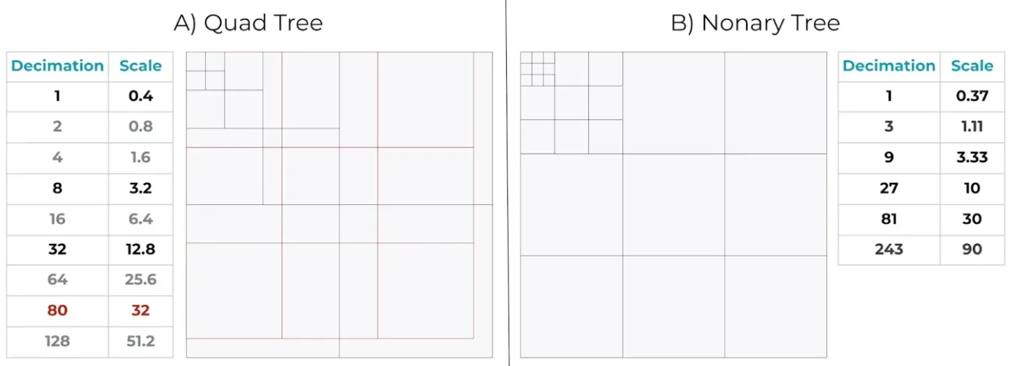
Figure 1. Comparison of quad tree (2x2) and nonary tree (3x3) grid hierarchies. A. Quad tree grids, with a base decimation of 2n, are a popular grid layout for web maps. But the quad decimated scales do not align particularly well with common satellite data pixel sizes. In this example, using 0.4 m as the base grid scale, there is no matching decimation to represent pixel sizes ~30 m (shown in red). B. Nonary tree grids, with a base decimation of 3n, better align with common satellite data pixel sizes.
A fundamental design decision concerns how resolution levels relate to one another. Most widely adopted Tile Matrix Sets are based on quad-tree structures with a factor-of-two decimation between zoom levels. Prominent examples include the WebMercatorQuad and WorldCRS84Quad TMS definitions. These systems work well for visualization and slippy-map use cases (Haklay and Weber, 2008, Dora, 2012), where smooth zoom transitions are important. However, factor-of-two steps do not align well with common EO spatial scales. Starting from a sub-meter base resolution, successive quad-tree decimation produces values that consistently miss frequently used scales such as 3 m, 10 m, and 30 m (Figure 1A). As a result, datasets must often be resampled to non-native resolutions when integrated into quad-tree–based TMS frameworks. This introduces interpolation artifacts and unnecessary storage overhead.
To better align with EO-native resolutions, we instead evaluated a nonary tree structure in which each tile is subdivided into a 3×3 grid at each zoom level. The resulting resolution progression closely approximates commonly used EO scales (Figure 1B). Starting from approximately 0.37 (10 / 33) m, successive levels produce values near 1 m, 3 m, 10 m, and 30 m without requiring irregular scaling factors. This reduces the need for repeated resampling when integrating data from multiple sensors. The nonary tree therefore provides a resolution ladder that is more naturally aligned with EO data analysis workflows than standard quad-tree–based TMS definitions.
Tile dimensions and internal block structure
Beyond resolution alignment, tile geometry must respect practical constraints imposed by storage formats and processing software. Larger tiles increase memory requirements, while smaller tiles increase orchestration overhead. Empirical testing indicated that tiles on the order of 4000 × 4000 pixels provide a good balance between memory footprint and scheduling overhead in distributed environments.
Tile dimensions and internal block structures must consider the extrinsic constraints imposed by the raster tooling used in geospatial production workflows. GeoTIFF, as implemented via GDAL, requires internal block dimensions that are divisible by 16 (Rouault et al., 2024). In practice, 512×512 pixel blocks are widely supported, efficient for cloud-native IO, and compatible with Cloud Optimized GeoTIFFs. Designing a grid around these dimensions ensures compatibility with existing tooling while preserving IO efficiency and memory safety on cloud computing resources.
For simplicity and for a better internal tile layout we dismissed the idea of non-square tiles early on in the design process.
Hierarchical indexing and tile encoding
In distributed raster systems, the tile identifier functions not only as a name but as a spatial index, a metadata key, and often a partitioning mechanism in object stores. Its structure therefore directly affects system complexity and performance. The tile index for a grid should be designed as a core component rather than a secondary labeling scheme.
Several existing hierarchical spatial indexing systems informed our design, most notably geohash (Niemeyer 2008), S2 (S2 Geometry Developers n.d.), and H3 (Brodsky 2018). All three encode spatial hierarchy and support efficient containment and locality queries, but differ in their subdivision strategies and encoding schemes. Geohash recursively subdivides latitude–longitude space and represents hierarchy using prefix-based strings. S2 partitions the sphere into a quad-tree of projected cube faces and encodes cell identifiers as hierarchical binary integers following a Hilbert space-filling curve. H3 uses a hierarchical hexagonal tessellation represented by a fixed 64-bit index. While these systems provide elegant spatial indexing for point and geometry queries, they were not designed for raster-native processing or alignment with EO resolution hierarchies.
From these systems we adopted several design principles. From geohash we adopted the use of hierarchical string encodings and prefix-based containment. From S2 and H3 we adopted the principle that the identifier should explicitly encode spatial hierarchy rather than require it be inferred. We did not adopt binary encodings, as our goal was to produce an index that remains human-readable while aligning directly with the nonary tree and the raster grid.
Based on these precedents, the following requirements were developed to guide the tile index design.
- The identifier must encode both resolution depth and spatial hierarchy in a single value. Parent–child relationships should be structurally encoded and apparent.
- The index should support prefix-based containment. It should be possible to determine ancestry and containment using simple string operations, enabling efficient prefix scans in key-value stores without spatial queries.
- The identifier should be compact and human-readable. While machine efficiency is important, operational workflows benefit from identifiers that can be inspected and reasoned about directly.
- The index must align with the nonary tree, reflecting its 3×3 subdivision pattern.
The indexing scheme derived from these requirements is described in the Results.
Results
Tile footprints of global projections
Equal-area projections produced the most compact tile grids. The Gall-Peters projection proved to be the most efficient, yielding the lowest tile count (568,980), which serves as the reference baseline for comparison (Table 1). The performance of the other equal-area projections was practically indistinguishable, all performing equally well. The compromise Plate Carrée reference system required 35.47% more tiles, while the Web Mercator and Peirce Quincuncial conformal projections required 105.38% and 116.92% more tiles respectively, reflecting large area distortions.
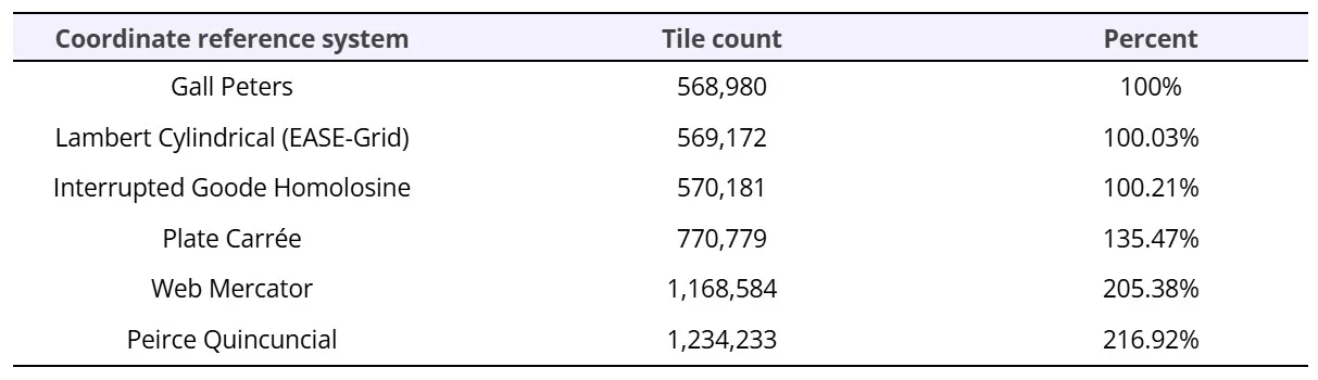
Table 1. Comparison of the total tile counts for six global reference systems corresponding to 4608 x 4608 pixels per tile at approximately 3 m pixel sizes. Relative tile count percentages are reported as the fraction of tiles for each projection relative to the reference system with the lowest tile count, Gall Peters.
Shape and area distortions
Equal-area projections preserved area but introduced angle and shape distortions (Figure 2, Figure 3). EASE-Grid showed systematic angular distortions that increased with latitude (Figure 2A), while Gall–Peters exhibited slightly lower angular variability among equal-area candidates (Figure 2B). Plate Carrée distorted both area and shape (Figure 2E). Conformal projections preserved local shapes but created substantial area distortions, especially for northern latitudes in Web Mercator (Figure 2C). Except for Interrupted Goode Homolosine (Figure 2D) and Peirce Quincuncial (Figure 2F), distortion patterns were systematic and primarily latitude-dependent. Peirce Quincuncial showed particularly excessive area and angle distortions in parts of Oceania, while angle distortions for Interrupted Goode Homolosine were most prevalent in areas near the discontinuities.
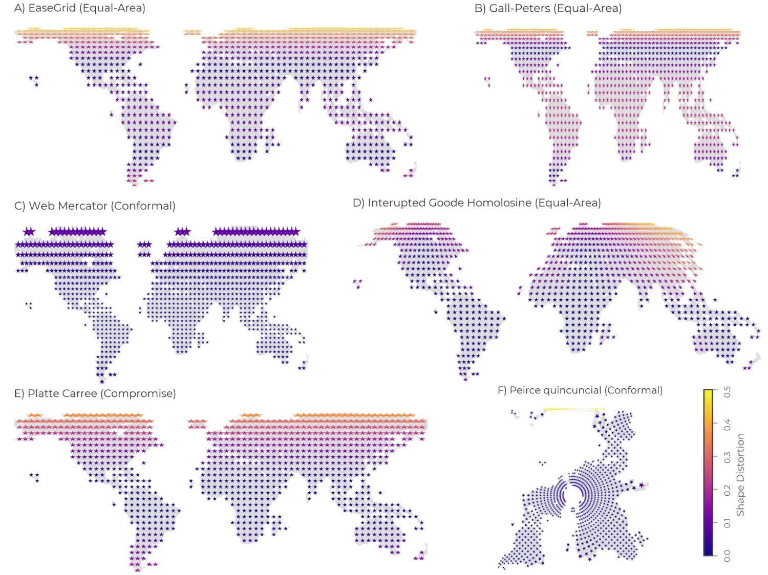
Figure 2. Area, angular, and shape distortions for six global coordinate reference systems visualized using equal area, north-facing pentagrams. Area distortion is represented by the size of each pentagram. Shifts in pentagram direction show angular distortion. Shape distortion is represented by pentagram color, with the gradient from dark blue to light yellow representing a gradient of low to high shape distortion.
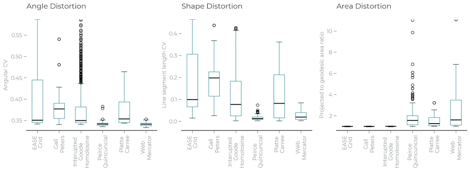
Figure 3. Bar plots comparing geometric distortions show the relative angle, shape, and area distortions introduced by six global coordinate reference systems. Equal-sized pentagrams were distributed every 5° over land and reprojected to each reference system. (A) Angle distortion was quantified as the coefficient of variation (CV) for all angles in each pentagram, (B) shape distortion as the line length CV for each segment in each pentagram, and (C) area distortion as the ratio of the projected area divided by the geodesic area for each pentagram. EASE Grid shows low average angle and shape distortions among equal area candidates, with long tails corresponding to greater distortions at high latitudes.
Coordinate reference system selection
Gall–Peters performed favorably in the quantitative evaluation due to its strong area-preserving properties and comparatively low angular distortion among equal-area projections. However, its lack of a standardized EPSG identifier introduced a significant operational drawback. In distributed systems, relying on explicit PROJ strings or WKT definitions increases configuration complexity and the risk of inconsistencies across environments. This limitation reduced its practicality despite its geometric performance.
Web Mercator performed well in several evaluation categories, particularly with respect to grid regularity. The square projected extent of conformal projections simplifies tiling, as it avoids the need to handle partially out-of-bounds tiles that arise in rectangular or asymmetric extents. However, the substantial area distortion at higher latitudes resulted in a dramatically larger pixel footprint. The associated storage and computational costs ultimately outweighed the benefits of Web Mercator’s clean tiling geometry.
Operational usability is critical in production contexts. EASE-Grid, Plate Carrée, and Web Mercator have established EPSG identifiers and broad support across GDAL, PROJ, and cloud-native tooling. In contrast, Gall–Peters lacks a standardized registry entry, Peirce quincuncial requires more recent PROJ versions, and Interrupted Goode introduces discontinuities that complicate tiling logic and indexing. Projections with strong tooling support reduce long-term maintenance effort and integration risk in distributed systems.
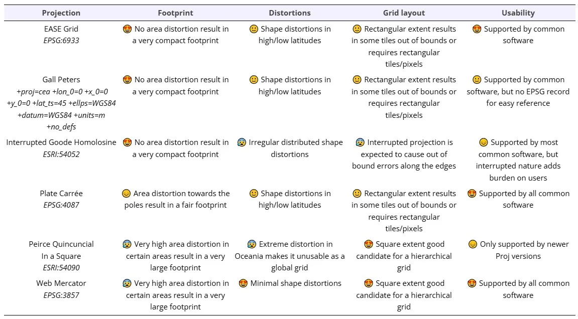
Table 2. Qualitative evaluations of grid layout, footprint, distortions, and usability for each of the global coordinate reference systems. Each evaluation metric is scored using emojis and described in text. EASE Grid strikes the best balance across each of these evaluation criteria, with no metric receiving a “poor” score while scoring “excellent” on usability and layout. Legend: 😰Poor, 😔fair , 🙂good, 😍excellent.
Projection, grid hierarchy, and tile dimensions
EASE-Grid was selected as the final projection. While it introduces systematic geometric distortion that increases with latitude, the distortion is predictable and acceptable for area-based land cover analyses. The rectangular extent results in some tiles extending beyond valid data boundaries, but these edge cases can be handled consistently within the tiling framework. Given its compactness, operational stability, and compatibility with existing tooling, EASE-Grid provided the most balanced solution for our workload.
- CRS: EPSG:6933
- Projected extent:( -17367530.44, -27612800.73, 17367530.44, 7122260.16)
- Geographic extent: (-180, NaN, 180, 76)
- Tile shape: 4,608×4,608
- Internal tile shape: 512×512
To ensure seamless global coverage without gaps or slivers at tile boundaries, the theoretical “ideal” pixel sizes had to be slightly adjusted (Table 2). Exact hierarchical divisibility and full extent coverage required adopting the following resolutions: 0.38 m, 1.15 m, 3.45 m, 10.34 m, and 31.02 m. These values remain sufficiently close to common EO resolutions of 0.3 m, 1 m, 3 m, 10 m, and 30 m that the differences are minor in practice, especially compared to the mismatches introduced by binary tree layouts (Figure 1). The exact divisibility adjustment guarantees consistent tile alignment across zoom levels over the full spatial extent, eliminating cumulative rounding errors at tile boundaries.
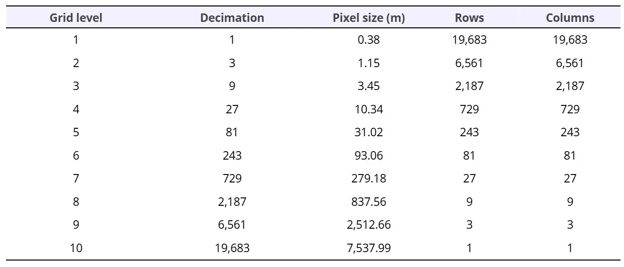
Table 3. Hierarchical grid specification describing pixel and tile sizes at each level in the 3n based nonary tree. The nonary structure provides clear alignment with standard satellite EO resolutions at grid levels 1-4. The values for pixel size were rounded to two decimal places.
Given that the EASE Grid extent is rectangular, we defined the width and height of the square grid using the east-west extent of the EASE Grid projection. Instead of centering the grid around the 0/0 coordinate, we added a negative offset along the y axis to snap the upper bound of the grid to the 76° northern parallel, which excluded the northernmost part of the Arctic Circle. The lower bounds were extended beyond the valid geographic extent. Specifying coordinates south of -90 simply defines a square grid; no data from these areas are produced.
The selected tile size of 4,608×4,608 pixels reflects extrinsic constraints imposed by existing geospatial production software. To remain compatible, tile size had to be divisible by 512. The 4608 dimension (9 × 512) allows a 9×9 internal block structure of 512×512 blocks, which mirrors the nonary tree structure up to three levels within a single tile (Figure 4). This constraint limited the depth of nonary subdivision that could be represented internally within one file. However, in practice, workflows rarely traverse more than two to three resolution levels in a single processing step, making this limitation acceptable.
Hierarchical indexing and tile encoding
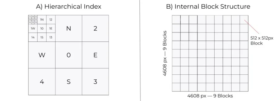
Figure 4. Tile index and block structure layouts for the grid specification. (A) The hierarchical index shows the nested index labels at progressively finer resolutions in the upper left tiles. (B) Each tile is organized with 4,608 by 4,608 x/y dimensions, and 512 x 512 internal block sizes. This internal block structure layout mirrors the 9 by 9 organization of the nonary grid.
We adopted a prefix-based encoding aligned directly with the nonary tree rather than the recursive binary subdivision used by geohash or the fixed-length 64-bit representation used by H3. Like geohash and H3, the index encodes hierarchical structure explicitly; unlike H3, it does not rely on opaque fixed-width binary integers, and it does not derive from alternating latitude–longitude bisection. Instead, the encoding reflects the 3×3 subdivision pattern of the nonary tree.
Each tile identifier represents the traversal path from the root to a leaf. At every 3×3 subdivision step, a single character is appended to indicate which of the nine child cells is selected:
- 0 denotes the center cell;
- 1–4 represent the four corner cells;
- and N, E, S, and W represent the edge cells.
The length of the resulting string corresponds directly to resolution depth (Figure 4A). Parent tiles are obtained by truncating the final character, and shared prefixes indicate shared ancestry within the tree.
This structure preserves the key hierarchical properties demonstrated by both geohash and H3—explicit multi-resolution encoding and structurally embedded ancestry—while maintaining human readability. The identifier simultaneously functions as a unique tile ID, a hierarchical spatial index, and a metadata partitioning key.
Importantly, the index remains fully compatible with conventional (z, x, y) Tile Matrix Set addressing. Because each character represents a deterministic subdivision within a known 3×3 layout, translation between the nonary index and a (z, x, y) representation is straightforward. The resolution depth maps directly to z, and cumulative child selections determine x and y positions. As a result, the grid can interoperate with standard TMS tooling while benefiting from a more expressive hierarchical identifier.
Compared to (z, x, y) addressing, hierarchical relationships are encoded directly rather than inferred. Containment reduces to prefix comparison, proximity can be approximated through shared ancestry, and metadata retrieval can be implemented efficiently via prefix scans in key-value stores. Resolution depth is implicit in the identifier itself.
When defining the index structure, we intentionally omitted grid level 0 and began indexing at level 1, which consists of the nine base tiles. Including level 0 would have resulted in all identifiers sharing the same leading character (0), adding no informational value while increasing string length. In practice, level 0 tiles are used only for coarse overviews such as thumbnail rendering and are not part of analytical workflows. Starting at level 1 therefore simplifies the index without reducing functionality.
Discussion
This work presents a nonary tree–based global grid designed specifically for cloud-native EO processing. By aligning resolution levels with common EO scales and selecting a projection that minimizes pixel footprint, while remaining operationally practical, this grid reduces unnecessary resampling and stabilizes compute and storage costs. The prefix-based index encodes hierarchy directly in the tile identifier, simplifying containment checks and enabling efficient metadata management in distributed systems.
We emphasize that this grid is not intended as a universal solution. Projection choice, resolution progression, and indexing strategy are inherently dependent on workload characteristics, geographic scope, and tooling constraints. Teams mapping Arctic areas might benefit from adopting the nonary tree layout while using the Northern Hemisphere Azimuthal EASE Grid projection, EPSG:6931, for example. The primary contribution of this paper is the structured approach to grid design: explicitly evaluating resolution alignment, distortion tradeoffs, pixel footprint, software compatibility, and operational impact before committing to an implementation. Below, we review some of the limitations of this implementation and discuss considerations for future grid designs.
Limitations
This grid introduces several tradeoffs:
- Pixel sizes are slightly offset from nominal EO resolutions
- Internal hierarchical depth is constrained by raster block size requirements
- Shape distortion increases with latitude
- Some tiles fall outside of the valid projection extent
These limitations were considered acceptable in exchange for reduced pixel footprint, predictable compute cost, and improved operational simplicity.
Distortion considerations in practice
EASE-Grid introduces systematic angular distortion that increases with latitude. In our evaluation, these distortions were predictable and monotonic rather than irregular or discontinuous. While geometric deformation is an inherent tradeoff of equal-area projections, its practical impact depends strongly on workload characteristics.
Our primary applications are predominantly area-based analyses, such as land cover mapping and zonal statistics, where consistency in pixel area is more critical than strict preservation of local shape. In such workflows, equal-area properties ensure that each pixel represents a consistent ground area across latitudes, stabilizing computational load and supporting meaningful spatial aggregation. From this perspective, predictable angular distortion is less consequential than uncontrolled variation in pixel density.
In contrast, shape distortion becomes more relevant in workflows that rely heavily on vision-based models for tasks such as fine-grained feature extraction or geometric pattern recognition. In these cases, angular deformation may influence how spatial patterns are represented at different latitudes, potentially affecting feature consistency and model transferability.
A central challenge in geospatial machine learning is generating reliable predictions beyond the spatial bounds of available training data. Such generalization depends on understanding distribution shifts between training and inference domains (Meyer & Pebesma, 2022). Under EASE Grid, angular distortion varies systematically with latitude; consequently, the latitudinal distribution of training data influences the extent to which inference remains in-distribution. While this interaction was not explicitly quantified in this study, the distortion pattern is structured and predictable, which may be preferable to irregular deformation introduced by interrupted projections.
Given our operational focus, the reduction in pixel footprint and improved stability of compute and storage costs outweighed the potential impact of systematic angular distortion. For area-centric analytical workflows, the equal-area property provided a more direct and measurable benefit than conformal geometry.
Internal structure constraints
The nonary tree is not natively supported by common raster formats. GeoTIFF requires internal block sizes divisible by 16 and efficient cloud-native access patterns strongly favor 512×512 blocks. These constraints are extrinsic to the grid design but non-negotiable in practice, limiting the internal representation of the nonary tree to three levels within a single 4608×4608 tile. Deeper hierarchical relationships are expressed across tiles rather than within a single file.
In operational terms, this limitation is rarely binding. Production workflows typically do not traverse more than two or three zoom levels within a single processing step. The chosen tile size therefore balances theoretical elegance with compatibility and IO efficiency.
Grid extent and offset adjustment
The native EASE-Grid extent is wider in the east–west direction than in the north–south direction. Consequently, hierarchical tiling produces cells that extend beyond the valid land extent, particularly at lower zoom levels where tiles cover large spatial areas. Other TMS-based systems, such as WorldCRS84Quad, mitigate this issue by starting with a 2×1 matrix at level 0 to reduce out-of-bounds cells (Masó et al., 2022). This approach was not suitable for our grid, as it conflicted with our resolution alignment and internal tile layout requirements.
We therefore accepted the presence of partially empty tiles. In practice, these tiles are clipped to the valid projection extent prior to writing. Clipping prevents reprojection errors due to out of bound pixels and ensures stable software behavior. As a result, the effective data footprint of such files may be smaller than the nominal tile extent. Tiles that fall entirely outside the projection domain are not written.
A further practical consideration arises from common library assumptions. Many software tools expect the (0,0) tile—defined as the top-left tile at a given zoom level in a Tile Matrix Set—to exist and attempt to retrieve metadata from it (Rouault et al., 2024). To ensure predictable behavior across client implementations, we introduced a vertical offset to the grid so that the upper-left corner aligns with 180°W and 76°N. This guarantees that the (0,0) tile at every zoom level lies within a valid spatial extent.
Operational impact
Adopting the grid significantly reduced cognitive and operational overhead. All raw data are reprojected onto the grid before entering production pipelines. This eliminates recurring discussions about resolution alignment, tiling strategy, and naming conventions. The grid provides a single canonical spatial reference for both data producers and consumers.
The Tile Matrix Set definition makes the grid consumable by existing open-source tooling (see Data Availability section). The prefix-based index enables efficient metadata lookup in key-value stores without requiring spatial database queries. Parent–child relationships are resolved via prefix operations, simplifying distributed metadata management.
Emergent use cases
Beyond its original purpose as a processing grid, the nonary tree structure enabled additional workflows. Training data sampling was aligned to grid cells, ensuring that each sample corresponds to exactly one tile and that tiles do not overlap across samples. This provides a simple mechanism to enforce geographic separation for spatially explicit train/test splits and reduces leakage between adjacent samples. The hierarchical index also enabled deterministic train/test splits by applying rules to the final character of the identifier. Because spatial hierarchy is encoded directly in the tile ID, such partitioning can be implemented without geospatial queries.
In change detection experiments, the nonary sibling structure proved useful for contextual analysis. The center cell (0) can be treated as foreground while its eight siblings provide neighboring spatial context. This pattern emerged naturally from the grid layout rather than being explicitly designed for that purpose.
Conclusion
Global raster processing at scale requires more than distributed compute; it requires disciplined spatial partitioning. While tiling is a well-established concept, the choice of grid structure, projection, and indexing scheme has significant downstream implications for computational efficiency, storage cost, model behavior, and operational complexity.
Interoperability was a central design principle. By expressing the grid as a 3×3 Tile Matrix Set and ensuring compatibility with widely adopted standards and tooling—such as GDAL, PROJ, Cloud Optimized GeoTIFF, and Zarr—we prioritized ease of adoption over theoretical optimality. In production environments, alignment with common standards is often more critical than marginal improvements in distortion metrics.
We hope that the framework presented here—defining clear design requirements, evaluating projections quantitatively, and grounding decisions in operational constraints—can serve as a template for others developing grids tailored to their own large-scale raster workflows. Thoughtful spatial partitioning is foundational infrastructure, and investing in its design yields compounding benefits across data production, analysis, and machine learning systems.
Acknowledgments
The authors thank the other members of the Forest Ecosystems team at Planet for testing the implementation in practice. The findings and views described herein do not necessarily reflect those of Planet Labs PBC.
Funding Information
This work was supported by Planet Labs PBC.
Author Contributions
Thomas Maschler: conceptualization, analysis, software, writing – original draft
Ryan McCarthy: conceptualization, software, writing – review & editing
Christopher Anderson: conceptualization, formal analysis, supervision, writing – review & editing
Data Availability
All data and code can be found here.
Transparent Peer Review
Results from the Transparent Peer Review can be found here.
Recommended Citation
Maschler, T., R. C. McCarthy, and C. B. Anderson. 2026. A cloud-native, compute-optimized tile grid for land cover analysis. Stacks Journal: 26010. https://doi.org/10.60102/stacks-26010
References
Afgan, E., and P. Bangalore. 2008. Embarrassingly parallel jobs are not embarrassingly easy to schedule on the grid. 2008 Workshop on Many-Task Computing on Grids and Supercomputers, 1–10. https://doi.org/10.1109/MTAGS.2008.4777910.
Basaraner, M., and S. Cetinkaya. 2019. New measures for analysis and comparison of shape distortion in world map projections. Cartography and Geographic Information Science 46: 518–31. https://doi.org/10.1080/15230406.2019.1567394.
Bauer-Marschallinger, B., and K. Falkner. 2023. Wasting petabytes: A survey of the Sentinel-2 UTM tiling grid and its spatial overhead. ISPRS Journal of Photogrammetry and Remote Sensing 202: 682–90. https://doi.org/10.1016/j.isprsjprs.2023.07.015.
Bauer-Marschallinger, B., D. Sabel, and W. Wagner. 2014. Optimisation of global grids for high-resolution remote sensing data. Computers & Geosciences 72: 84–93. https://doi.org/10.1016/j.cageo.2014.07.005.
Brodsky, I. 2018. H3: Uber’s hexagonal hierarchical spatial index. Uber Blog. June 27. https://www.uber.com/en-EG/blog/h3/.
Brodzik, M. J., B. Billingsley, T. Haran, B. Raup, and M. H. Savoie. 2012. EASE-Grid 2.0: Incremental but significant improvements for earth-gridded data sets. ISPRS International Journal of Geo-Information 1: 32–45. https://doi.org/10.3390/ijgi1010032.
Buchwal, A., G. Rachlewicz, B. Heim, and B. Juhls. 2023. Trees on the tundra: Warmer climate might not favor prostrate Larix Tree but Betula nana shrub growth in Siberian tundra (Lena River Delta). Agricultural and Forest Meteorology 339: 109543. https://doi.org/10.1016/j.agrformet.2023.109543.
Della Dora, V. 2012. A world of ‘slippy maps’: Google Earth, global visions, and topographies of memory. Transatlantica: Revue d’Études Américaines. American Studies Journal. https://doi.org/10.4000/transatlantica.6156.
Gargantini, I. 1982. An effective way to represent quadtrees. Communications of the ACM 25: 905–10. https://doi.org/10.1145/358728.358741.
Gibb, R. G., M. B. J. Purss, Z. Sabeur, P. Strobl, and T. Qu. 2022. Global reference grids for big earth data. Big Earth Data 6: 251–55. https://doi.org/10.1080/20964471.2022.2113037.
Goodchild, M. F. 2000. Discrete global grids for digital earth. Specialist Research Meetings—Papers and Reports: 69–77. https://escholarship.org/uc/item/4tm0d1jm.
Grafarend, E. W. 1995. The optimal Universal Transverse Mercator projection. Manuscripta Geodaetica 20: 421–68. https://doi.org/10.1007/BF03655477.
Haklay, M., and P. Weber. 2008. OpenStreetMap: User-generated street maps. IEEE Pervasive Computing 7: 12–18. https://doi.org/10.1109/MPRV.2008.80.
Kmoch, A., I. Vasilyev, H. Virro, and E. Uuemaa. 2022. Area and Shape Distortions in Open-Source Discrete Global Grid Systems. Big Earth Data 6: 256–75. https://doi.org/10.1080/20964471.2022.2094926.
Lewis, A., S. Oliver, L. Lymburner, et al., 2017. The Australian geoscience data cube—Foundations and lessons learned. Remote Sensing of Environment 202: 276–92. https://doi.org/10.1016/j.rse.2017.03.015.
Masó, J., J. Yutzler, P. Rushforth, J. Jacovella-St-Louis, and J. Harrison. 2022. OGC Two dimensional tile matrix set and tile set metadata. Version 2.0. Open Geospatial Consortium. http://www.opengis.net/doc/IS/tms/2.0.
Meyer, H., and E. Pebesma. 2022. Machine learning-based global maps of ecological variables and the challenge of assessing them. Nature Communications 13: 2208. https://doi.org/10.1038/s41467-022-29838-9.
NASA Earth Science Data Systems. 2021. Data processing levels | NASA earthdata. Data Basics. Earth Science Data Systems, NASA. https://www.earthdata.nasa.gov/learn/earth-observation-data-basics/data-processing-levels.
Newman, D. J. 2024. Zarr storage specification. https://doi.org/10.5067/DOC/ESCO/ESDS-RFC-048V1.
Niemeyer, G. 2008. Geohash.Es. Geohash.Es – Geohash tools. https://www.geohash.es/.
Pollock, N. 2024. Cloud Optimized GeoTIFF (COG) File Format RFC. https://doi.org/10.5067/DOC/ESCO/ESDS-RFC-049V1.
Rouault, E., F. Warmerdam, K. Schwehr, A. Kiselev, H. Butler, M. Loskot, T. Szekeres, E. Tourigny, M. Landa, I. Miara, B. Elliston, K. Chaitanya, L. Please, D. Morissette, A. Jolma, N. Dawson, D. Baston, C. de Stigter, and H. Miura. 2024. GDAL. Version 3.9.2. Zenodo. https://doi.org/10.5281/ZENODO.13330875.
S2 Geometry Developers. n.d. S2 Geometry Library. Accessed July 15, 2026. https://s2geometry.io/.
Samet, H. 1984. The quadtree and related hierarchical data structures. ACM Computing Surveys 16: 187–260. https://doi.org/10.1145/356924.356930.
Sarago, V. 2026. Morecantile. Python. Version 7.0.3. Development Seed. https://github.com/developmentseed/morecantile.
Snow, A. D., M. Cochran, D. Hoese, I. Miara, J. Van den Bossche, C. Mayo, G. Lucas, P. Cochrane, J. de Kloe, C. Karney, J. Jimenez Shaw, T. Quoc Anh, F. Filipe, G. Ouzounoudis, B. Couwenberg, G. Lostis, J. Dearing, B. Jurd, C. Gohlke, C. Schneck, D. McDonald, M. Taves, M. Itkin, R. May, A. J. Stewart, H. de Bittencourt, B. Little, R. Hugonnet, P. Sai Rahul. 2025. Pyproj. Version 3.7.2. Zenodo. https://doi.org/10.5281/ZENODO.2592232.
Snyder, J. P. 1987. Map projections: A working manual. In Professional Paper, No. 1395. U.S. Government Printing Office. https://doi.org/10.3133/pp1395.
Stockinger, H., M. Pagni, L. Cerutti, and L. Falquet. 2006. Grid approach to embarrassingly parallel CPU-intensive bioinformatics problems. 2006 Second IEEE International Conference on E-Science and Grid Computing: 58. https://doi.org/10.1109/E-SCIENCE.2006.261142.
Open Access
Peer-Reviewed
Creative Commons
Submitted: 5 May 2026
Accepted: 7 July 2026
Published: 4 September 2026
This work was supported by Planet Labs PBC.
Conflicts of Interest:
All authors are employees of Planet Labs PBC, which funded this work.


