

How to avoid the camera trap: the effect of camera settings on occupancy analysis and photo data workload

Abstract photo. A gray fox pictured at a remote camera station.
Abstract
Camera traps (i.e., game cameras or trail cameras) have become a widespread tool in wildlife ecology. However, camera traps can take large volumes of photos or videos often generating a considerable data management workload. Internal camera settings, such as how many photos are taken when the camera is triggered and how long the camera waits before it can be triggered again, significantly influence the volume of photos collected. These settings have the potential to affect analytical results (e.g., estimated occupancy), photo management workload (i.e., reviewing and identifying images) and data storage requirements. Using two large baited camera trap datasets from California and Oregon (n = 1034 cameras), we compared effects of various internal camera settings (delay period = 5 – 300 seconds, burst number = 1 – 3) on occupancy and detection probabilities of three species ranging in body size and in occurrence from rarely to commonly detected [medium size-rare: Pekania pennanti (fisher), medium size-common: Urocyon cinereoargenteus (gray fox), large size-common: Ursus americanus (American black bear)]. We found increasing camera delay or decreasing burst number, both of which act to decrease photos taken, did not result in significant changes in detection probability or occupancy estimates for any of the three species analyzed. Cameras with the shortest delay and highest burst setting resulted in >1500% more photos compared to those with the longest delay and smallest burst setting without providing any analytical benefit for occupancy analyses. Our results demonstrate that when planning camera studies careful consideration of camera settings is needed to ensure data is collected efficiently to meet analysis objectives.
Keywords: burst, camera trap, detection probability, occupancy, photo interval, quiet period, trigger delay
Introduction
Camera trapping, or the deployment of heat- or movement-triggered cameras (also referred to as remotely triggered, game or trail cameras), has become ubiquitous around the globe for wildlife research and monitoring (O’Connell et al., 2011, Burton et al., 2015, Oliver et al., 2023, Goldstein et al. 2024a). Camera traps have gained popularity because they are relatively inexpensive, easy to deploy, and can passively survey for long periods with little or no human involvement for a wide range of taxa (Fisher, 2025). This has resulted in a dramatic increase in survey duration and temporal extent of camera trap studies over the last two decades (Steenweg et al., 2017, Delisle et al., 2021). For many studies that use camera traps, the aim is to collect photos that serve as an index of ecological processes (e.g., occupancy, abundance, distribution, biodiversity; Burton et al., 2015). However, these surveys can result in large numbers of photos which require significant data management time that is often not adequately accounted for in project planning. This problem is compounded by the fact that the majority of photos taken by camera traps are not species detections, but rather are misfires due to sun or vegetation movement in the background (Beery et al., 2019). Large photo management workloads can potentially hinder research and conservation by slowing the pace of projects due to the need to classify high volumes of images or result in incomplete and un-used datasets due to the lack of staff time to adequately process photos.
With the advent of machine learning, neural networks, and artificial intelligence (AI) based photo identification pipelines, there has been considerable progress in increasing photo management efficiency (Norouzzadeh et al., 2018, Ahumada et al., 2020). However, these advancements do not solve all aspects of photo management, nor do they completely negate the workload of processing high volumes of photos. Many field research environments have little to no internet connectivity and cannot rely solely on a cloud-based photo management system. In such cases, photographs are often stored and backed up on multiple laptops or hard drives, at least temporarily, until they can be fully processed. In the field, settings that increase photo numbers also can increase labor costs and time due to the need to more frequently service cameras that fill up memory cards or deplete batteries more quickly. In the office, high photo numbers increase required memory space on drives and time required for data transfer or image backup, which can become extensive when dealing with hundreds of thousands to millions of photographs. AI systems are not fully automated (Vélez et al., 2024) nor are they accurate for rare species without sufficient training data (e.g., Tuia et al., 2022). Thus, even when using AI technology significant human time is still required to upload photos, review, and confirm computer generated species identifications to prevent analytical bias generated due to mis-classification rates found in fully automated photo workflows (Longinser et al., 2024).
Several factors influence the number of photos a camera trap collects, some of which pertain to field conditions or study design, such as camera placement (e.g., camera angle, aspect, overhead cover, or surrounding vegetation) or survey duration, while others are dependent on internal camera settings. There has been extensive research on study design for cameras on factors such as camera model (Palencia et al., 2022), placement (Hofmeester et al., 2021), height (Jacobs and Ausband, 2018), effective survey area (Tucker et al., 2021), survey duration (Steenweg et al., 2016), and seasonality (Kays et al., 2020, Iannarilli et al., 2021). However, few studies have looked at how internal camera settings influence analytic results relative to photo management workload (Hamel et al., 2013, Lepard et al., 2019, Sparkes et al., 2021). In fact, many studies do not report internal camera settings in published papers (e.g. Apps & McNutt, 2018; Meek et al. 2015). Non-optimal camera settings that take too many photos greatly increase data management time and costs (Lepard et al., 2019). Conversely, camera settings that take too few photos could decrease detection of target species and compromise the ability to meet study objectives (Parker-Shames et al., 2024). Rare or hard to detect species with only fleeting presence at cameras may benefit from settings that trigger photos more rapidly compared to common species or easily detected species (e.g., Manley et al., 2004, Kristensen and Kovach, 2018), so taking too few photographs for such species could jeopardize conservation efforts. Despite the considerable influence camera settings can have on research objectives and data management, camera trap study design has to date principally focused on external factors such as number or spacing of cameras but there is little guidance on how best to optimize internal settings for specific research objectives.
While some aspects of camera performance are defined by the camera model and typically cannot be adjusted (e.g., trigger speed, trigger recovery time, field of view), others can be controlled by the user. Here we address two adjustable settings that control the number of photos taken and therefore photo management workload. First, the photo delay period (also referred to as trigger delay or quiet period, hereafter ‘delay’), is a period of dormancy after an initial motion- or heat-triggered photo when the camera will not take further photos regardless of motion or heat present. The delay setting can range from less than a second to hours and is used to reduce the number of photos and conserve battery life. Second, the burst setting (also referred to as rapid-fire or hyperfire number, hereafter ‘burst’) determines how many photos are taken in immediate sequence each time the sensor is triggered. Burst settings can range from 1 to as many as 100 photographs, depending on camera model. The time between successive burst photos is adjustable for some camera models but most often these burst photos are taken in rapid succession (<1 second between photos within a burst). Multi-photo bursts are thought to increase likelihood of detecting some species, particularly rapidly moving or otherwise hard to detect species. Increased bursts may be necessary for photo-based individual identification or measurements, especially if individuals have unique markings or features that can only be viewed from particular angles. From a data management perspective, both the burst and delay settings control the overall number of photos taken and could cause the same camera to take anywhere from dozens to tens of thousands of photos, and therefore have huge implications for data workload.
Camera trap data are often analyzed using occupancy analysis, which requires collating multiple photos of a species within a defined capture interval (e.g., 1 day, 1 week) into a single detection event (Mackenzie et al., 2002, Kellner et al., 2022). Because of this data structure, multiple photos of a species within the same capture interval do not change the occupancy estimate even though they increase photo review time and storage requirements. Therefore, for occupancy analyses seeking to inventory diversity or monitor common species, it might be assumed that a longer delay and low burst would be optimal. Conversely, if the goal of a study is to detect rare or elusive species, increasing confidence in the likelihood to detect such individuals is paramount. This presents a challenge to balance settings that provide increased photographs (low delay, high burst) versus reducing data management workload. This challenge is more pronounced with baited cameras, in which a food based reward or other attractant such as scent lure draws in and retains the animals in the camera frame for extended periods of time compared to unbaited cameras (Stewart et al., 2019, Dart et al., 2022).
While shorter delay settings may be beneficial for fine-scale analyses (e.g., activity patterns or individual identification) for other metrics, such as occupancy or relative abundance, longer delay settings may yield comparable results while greatly reducing data management needs. One prior study found increasing delay had a negligible effect on occupancy analyses for time-lapse cameras (Hamel et al., 2013). In another study Sparkes et al. (2021a) evaluated the effect of long camera delays (5 to 60 minutes) on relative abundance indices and found increasing delay reduced detection frequency but did not greatly affect results for delays up to 5 minutes. Lepard et al. (2019) found that increasing delay periods from 10 seconds to 10 minutes had only a small effect on occupancy estimates at unbaited cameras. However, these two latter camera trap studies were conducted with relatively small spatial extents (~<220 km2) with fairly common species and thus did not address the effect of camera settings on detecting rare species on large landscapes. Furthermore, none of these studies examined varying burst settings on analytic results or data management workloads.
To better understand the effect of delay and burst settings on occupancy analysis for baited camera traps at a landscape scale, we examined data from two large-scale camera trapping studies in California and Oregon, USA. These two studies were designed to monitor a rare carnivore, the fisher (Pekania pennanti). In the two study areas, the southern Sierra Nevada fisher population is listed as an endangered distinct population segment (DPS) under the Endangered Species Act (ESA) and the southern Oregon population has been petitioned multiple times for ESA listing as part of a separate DPS (USFWS, 2020, 2023). Due to the broad scale of these study designs, it enabled us to use the data for analysis of camera function with multiple species.
Because body size and rareness can both influence detectability (Tobler et al., 2008, Steenweg et al., 2019), we analyzed multiple species that varied in these characteristics. Fishers are a medium-bodied species whose populations have contracted in the western states from their historical range, and the species is considered rare. American black bears (Ursus americanus; hereafter, black bear) are common and large-bodied in these systems (Zielinski et al., 2005). Gray foxes (Urocyon cinereoargenteus) are common and medium-bodied and for our purposes, were a similar body size as fisher but differed in their greater relative abundance in our study areas. We considered including analysis of a large-bodied rare species, the mountain lion (Puma concolor) but we did not have sufficient detections to fit occupancy models for that species. Smaller bodied species were not analyzed as the camera protocols used were designed to detect medium-to-large-bodied carnivore species, and therefore, the camera sensors were not optimized to reliably detect small mammals. Our objectives were to assess how internal camera settings of delay and burst: 1) affect occupancy analyses estimates and precision; 2) interact with external factors, specifically body size, commonness and rarity of species on large landscapes; and 3) affect data management workload.
Methods and Materials
Field studies
We used data from two camera trapping studies with similar field protocols and species community composition. The first dataset was from the Southwest Oregon fisher study (hereafter Southwest Oregon) was conducted in 2016 and encompassed federal, state, and private forests in southwestern Oregon, and spanned ~64,000 km2 from the Cascade Crest to the Pacific Ocean (Figure 1). Camera deployments ranged from a mean of 43 days in summer (May – October) to 61 days in winter (January – March) and were checked at variable intervals depending on season and locality (Barry, 2018). Camera locations ranged from sea level to 2,286 m above sea level and were selected using a stratified random sample of a 9 km2 grid. We selected the grid size because it is the approximate size of a female fisher home range, and thus the recommended spacing for taxa-specific for occupancy models (Linden et al., 2017, Barry et al., 2021). This grid size is slightly larger than ideal for gray fox occupancy (home range: 0.67 – 5.45 km2; Jones, 2023) but is smaller than ideal for black bear (home range: 7.5 – 204 km2; Matthews et al., 2004). However, given that the objective of this paper was in analyzing camera settings not on the species occupancy estimates themselves this should not affect interpretation of results.
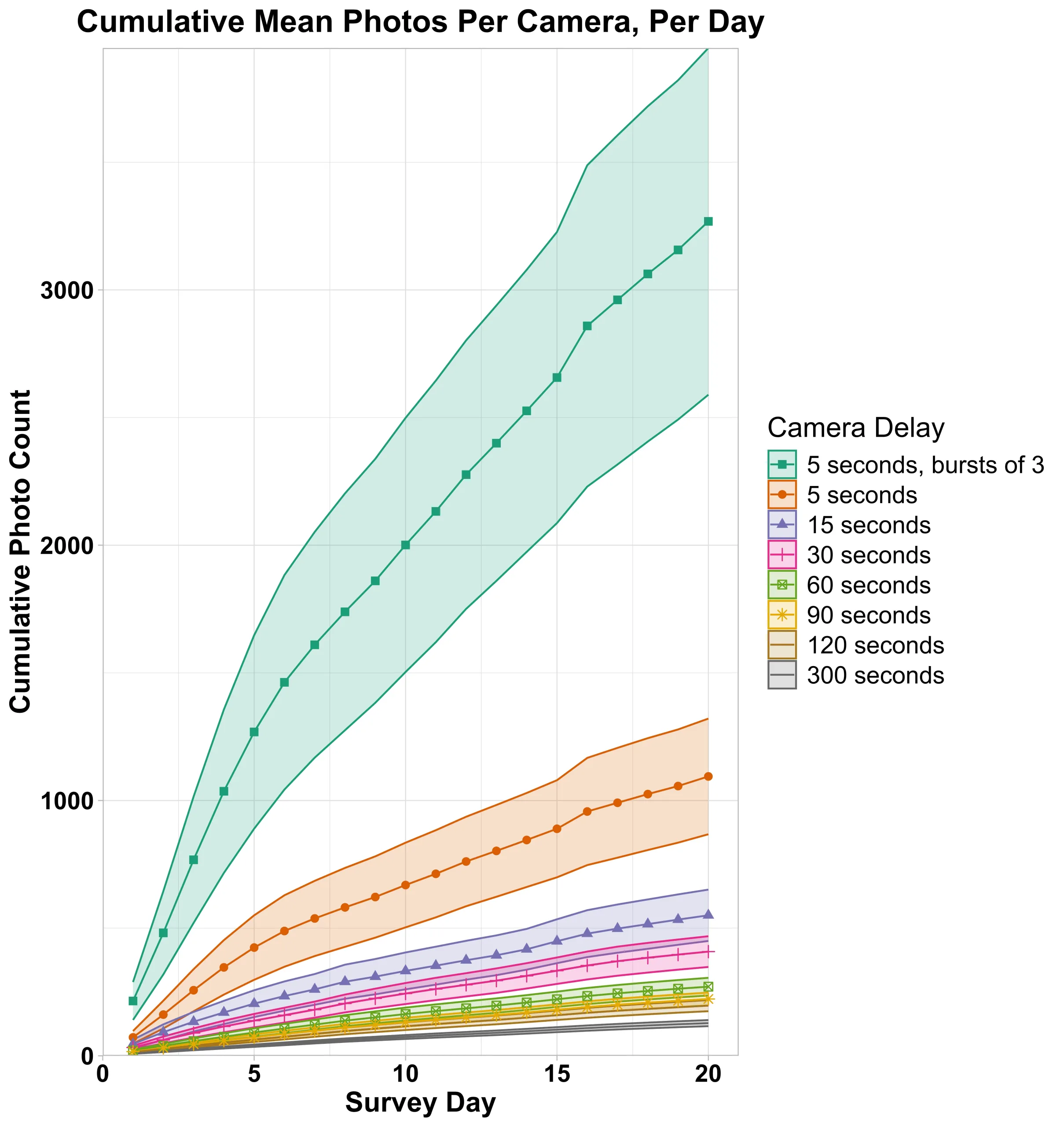
Camera stations were located in forest cover types within 1,000 m of a road or 250 m of a trail for accessibility. Sampling was conducted using device arrays at each location (together considered one sample unit; Evans et al., 2019, Anderson et al., 2023). Within each selected cell, three cameras were placed 1,000 m apart in a triangle centered on a randomized point. Each camera was deployed with a scent lure (Gusto, Minnesota Trapline Products, Pennock, MN, USA) and a randomized bait type (raw chicken, cat food, or a multi-bait ‘kitchen sink’, see Barry et al., 2021). A fourth additional un-baited camera was set near a trail or road within 150 m of the northernmost baited camera. For the purpose of this study and because the number of unbaited cameras deployed was small, we only analyzed results from baited cameras (N = 286 cameras from N = 106 sample units). Cameras were set to a 5 second delay with a 3-photo burst. Camera models used included Browning Dark Ops HD (Morgan, UT, USA) and Bushnell Aggressor No Glow (Overland Park, KS, USA).
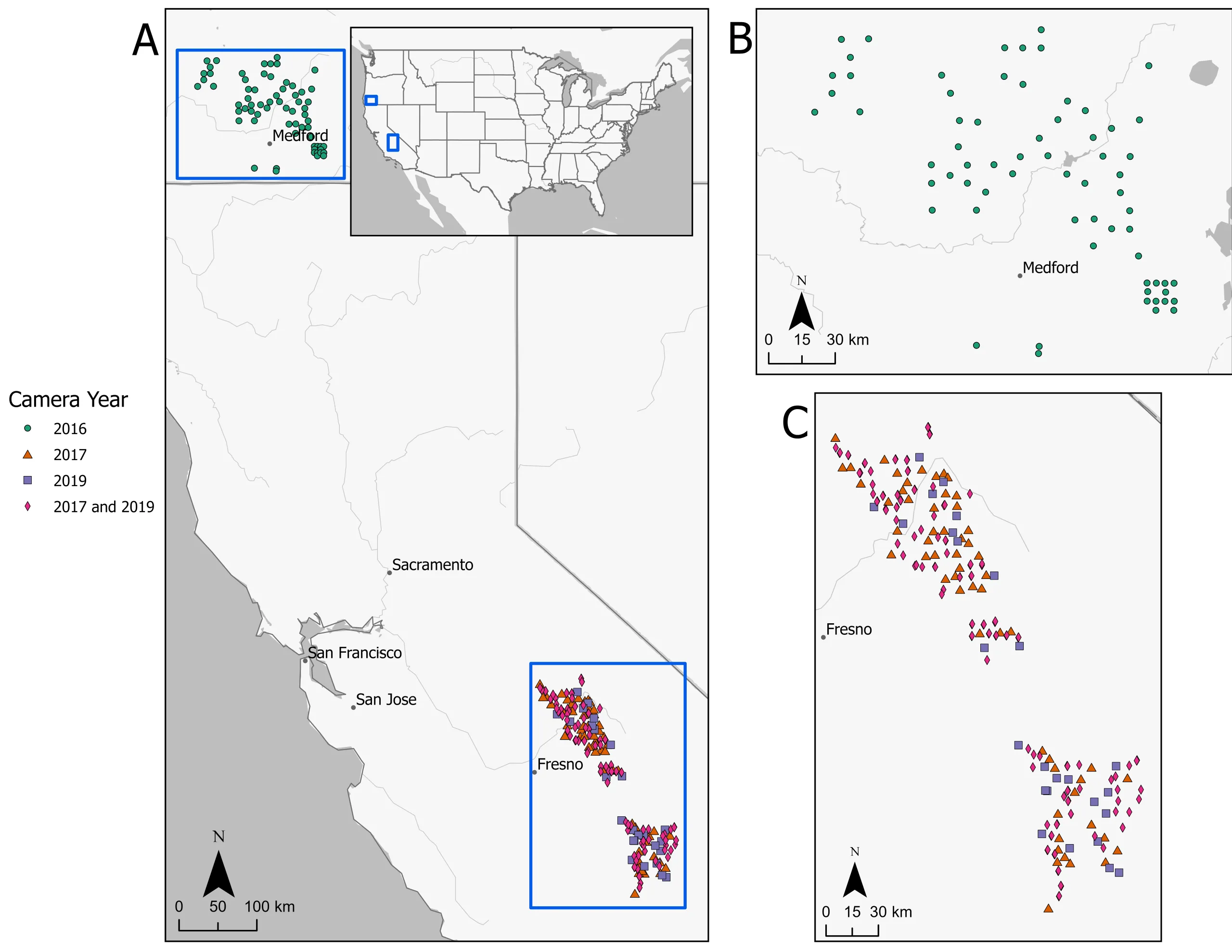
The second study was part of the United States Forest Service (USFS) Sierra Nevada Carnivore Monitoring Program (hereafter, Sierra Nevada) which surveys primarily USFS lands on the western slope of the Sierra Nevada Mountains south of Yosemite National Park (Figure 1; Zielinski et al., 2013), CA, USA. Sampling occurred annually across ~12,000 km2 from June to October with survey sites ranging from 1,000 to 3,400 m elevation above sea level. Sampling units were co-located with USFS Inventory and Analysis (FIA) plots in a variety of habitat types that contained potentially suitable forest cover (e.g. excluding non-forested areas such as grasslands and urban areas). Sample units consisted of three baited cameras deployed in a triangle ~500 to 800 m apart (Zielinski et al., 2017). Devices were baited with raw chicken and a commercial trapping lure (Gusto, Minnesota Trapline Products, Pennock, MN, USA). Each device was checked and rebaited 3 times approximately every 7 days for an average deployment of 21 days. We analyzed data from two years that had different delay periods to compare the settings (2017 = 30-second delay, 2019 = 15-second delay). All other camera settings and models were consistent among years (burst = 1, models = Bushnell Trophy Cam, Trophy Cam HD, Essential, and Aggressor, all “No Glow” flash; Overland Park, KS, USA).
Photo processing
All photos were individually identified and ‘tagged’ with metadata including species or, for images with no wildlife species detections, as ‘crew’ (field crew present in the photo), ‘blank’ (no wildlife present), or ‘inoperable’ (camera malfunction). For the Southwest Oregon cameras with a 3-photo burst setting, each photo was individually tagged based only on the information visible in a single photo (i.e. other photos in the burst sequence were not used to aid identification). After photo tagging to facilitate tracking burst sequences for this analysis the photos were grouped using their timestamps and then each photo was identified with a burst number as either the first, second, or third photo in each burst sequence. Tagging ‘blank’ photos was essential, as false triggers also activate the camera delay period during which no additional photos are captured.
Delay and burst simulation
We organized the data into two datasets to address delay and burst effects separately. In the first dataset, to compare the effect of increasing delay settings, we standardized the Southwest Oregon dataset (burst = 3) to the Sierra Nevada datasets (burst = 1) by subsetting photos so only the first photo from each burst series was included in the dataset (simulating burst = 1 for all cameras). We then simulated the effect of changing the delay periods by subsetting our raw photo data with increasingly larger delay intervals (5, 15, 30, 60, 90, 120, 300 seconds) starting with the smallest delay interval for each of the datasets and subsetting to all larger delay intervals. For these simulations, after the first photo in a time sequence, we removed all subsequent photos within that delay period from the dataset, creating a separate dataset for each delay interval.
For the second dataset, to compare the effect of changing the burst settings, we used the 2016 Southwest Oregon camera data alone, as this was the only dataset that employed a multi-photo burst setting (burst = 3). We sequentially subset each photo burst to generate three photo datasets consisting of a) only the first photo, b) only the first and second photo, and c) all three photos from each photo burst.
Finally, for both datasets, we assessed the effect that various delay and burst settings would induce on photograph data management by calculating cumulative number of photos over 20-days and mean number of photos per day for each camera under the range of delay settings (5 – 300 seconds) and burst number (1 or 3).
Occupancy analysis
Occupancy models estimate site occupancy (ψ) while accounting for imperfect detection (p) by using repeated surveys at the same site (Mackenzie et al., 2002). We estimated ψ and p for black bear, gray fox, and fisher across a range of delay and burst settings to determine the effect of these settings on parameter estimates. Occupancy analyses were conducted separately for each species in R version 4.5.0 (RStudio Team, 2020, R Core Team, 2021) using the unmarked package (Fiske & Chandler, 2011).
We created 24-hour encounter histories for each camera station (0 = not observed, 1 = observed in >1 photo) such that each camera day was treated as a repeat survey (Davis et al., 2018, Rich et al., 2023). Because camera deployment times varied considerably between studies we standardized camera deployment length across projects by truncating all encounter histories to 20 days. We then fit encounter histories to single-season occupancy models without covariates via the occu function in unmarked. As our objectives were to assess the difference in estimates across different camera settings, we used intercept only models for detection and occupancy (ψ[.], p[.]). We then compared the resulting parameter estimates (ψ and p), and variation in these estimates (SE) across delay periods (5, 15, 30, 60, 90, or 300 seconds) and burst numbers (1, 2, or 3). Because each combination of study area and year used different delay settings (5, 15, 30 seconds) and numbers of cameras, combining all data into a single dataset would result in inconsistent sample sizes across delay periods. To keep sample sizes consistent to facilitate direct comparisons of SE between subset delay periods, we treated each combination study area and year as its own dataset and analyzed each independently (see Table 1 for camera sample sizes).
We conducted occupancy analyses at two different scales: individual cameras and a combined 2-camera sample unit for which we aggregated encounter histories across both cameras for analysis. We chose to analyze 2-camera units, despite a 3-camera unit protocol for both study areas, to ensure equal sample size across all units as, at many units, at least 1 of 3 cameras was missing due to a camera malfunction, black bear disturbance, or other field logistics problems. Therefore, we selected the first two numbered camera stations which were operational from each sample unit to aggregate for unit-level analyses.
Results
We assembled data from 1,034 camera stations resulting in 1,171,636 photos (Table 1). Mean photographs per camera per day ranged from 283 for the 2019 Sierra Nevada data (delay = 15 seconds, burst = 1) to 3,245 for the 2016 Oregon data (delay = 5 seconds, burst = 3). Interestingly, the 2019 Sierra Nevada dataset had a slightly lower average number of photos per camera (283 photos/day) than the 2017 dataset (404 photos/day) despite having a shorter delay period (15 vs 30 seconds). Upon further investigation, this was attributable to the 2017 dataset having more cameras with high photo counts due to extensive false triggers from background vegetation. The ratio of blank photos to species detections varied by year and project, but for all projects and years the majority of photos were blanks (68 – 75%) rather than species detections (16 – 29%).
Simulating an increased delay period for the Sierra Nevada camera data from 15 to 30 seconds resulted in a 36% decrease in photos, and photo number steadily decreased as the delay period increased with the maximum delay in our simulations (300 seconds) resulting in an overall photo reduction of 72-76% per year compared to a 15 second delay. For the Oregon data reducing 3 photo bursts down to a single photo resulted in a 66% reduction in photos. Further simulating an increased delay period (with burst = 1) from the original 5 second delay period reduced photos an additional 21% (15-second delay) to 80% (300-second delay). Over the 20-day survey period for the Oregon photos, we found a >1,500% increase in photos per camera when comparing the camera settings designed to take the most photos (delay = 5 sec, burst = 3, mean photos/camera = 3,245), compared to settings designed to take the least photos (300 sec, burst = 1, mean photos/camera = 214; Figure 2).
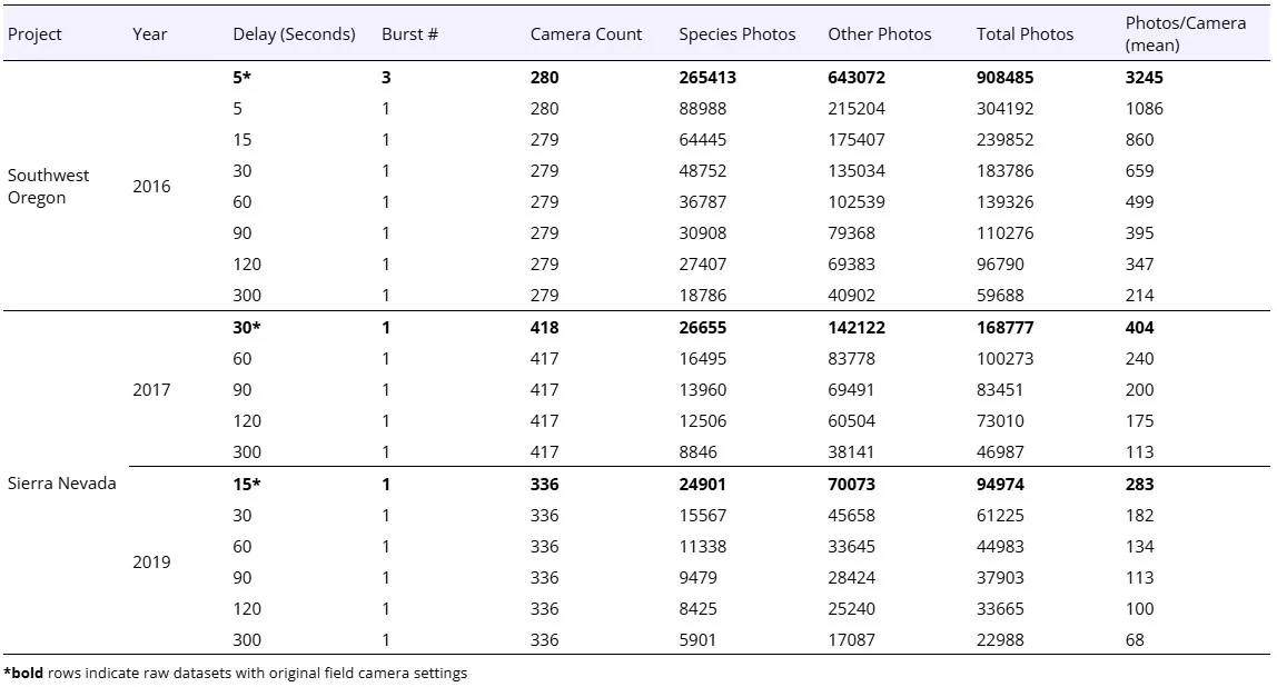
Table 1. Photo counts for each study area by year for a 20-day survey period for the original dataset (denoted with bold*) and each data subset simulating increasing delay periods. Species photos include photos of any wildlife species detected. Other photos include blanks and photos of crew members or vehicles.
Delay simulation
Parameter estimates for occupancy and detection were generally consistent across delay periods for all species across the three datasets. Parameter estimates for a single camera were either equivalent or only showed minor variation across delay periods for all datasets analyzed, with a maximum observed variation in ψ of ± 0.03 or a maximum variation in p of ± 0.02. The largest variation in ψ was observed in the Southwest Oregon fisher data (ψdelay5 = 0.05 [SE = 0.02], ψdelay300 = 0.03 [SE = 0.02]) and 2017 Sierra Nevada black bear data (ψdelay5 = 0.70 [SE = 0.02], ψdelay300 = 0.67 [SE = 0.03]). Variation around parameter estimates (SE) for single cameras was minor (>± 0.01) across all delay periods and datasets (Figure 3, Table S1). These results were consistent for analyses of 2-camera units (Table S2).
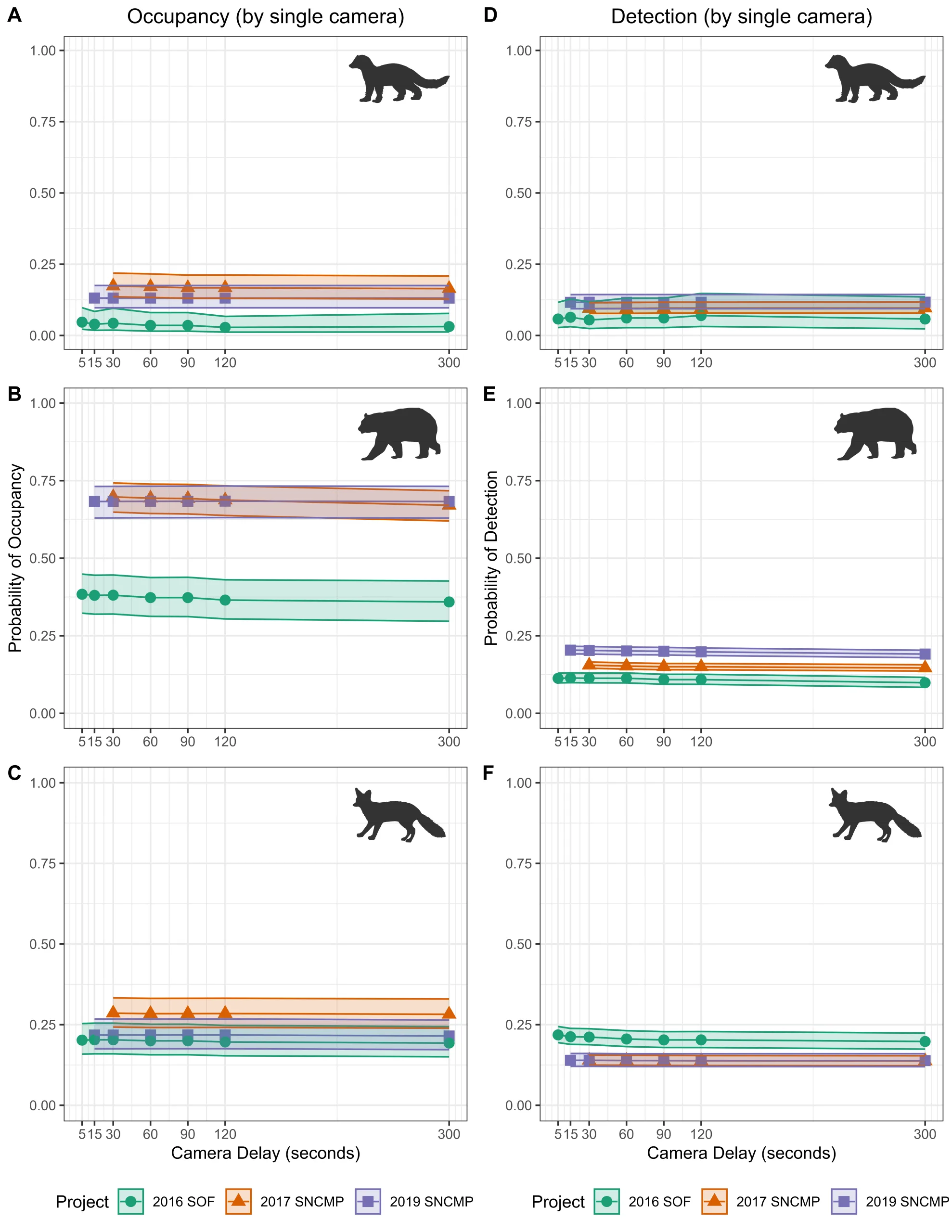
Figure 3. Plots of (A – C) occupancy and (D – F) 24-hour detection probability by species for a single camera for each of the raw datasets: Sierra Nevada Carnivore Monitoring Project (S. Nevada) in 2017 (green circles) & 2019 (orange triangles) and the Southwestern Oregon Fisher project (SW Oregon) in 2016 (purple squares). Species results are organized by row: Row 1 = fisher, Row 2 = black bear, Row 3 = gray fox. The original delay period varied by study area and year (SW Oregon 2016 = 5 sec, S. Nevada 2017 = 30 sec, S. Nevada 2019 = 15 sec).
Burst simulation
When analyzing the effect of changing the burst number in occupancy analyses, there was no effect of changing burst number on either the parameter estimates ψ or p, or their standard errors (Figure 4).
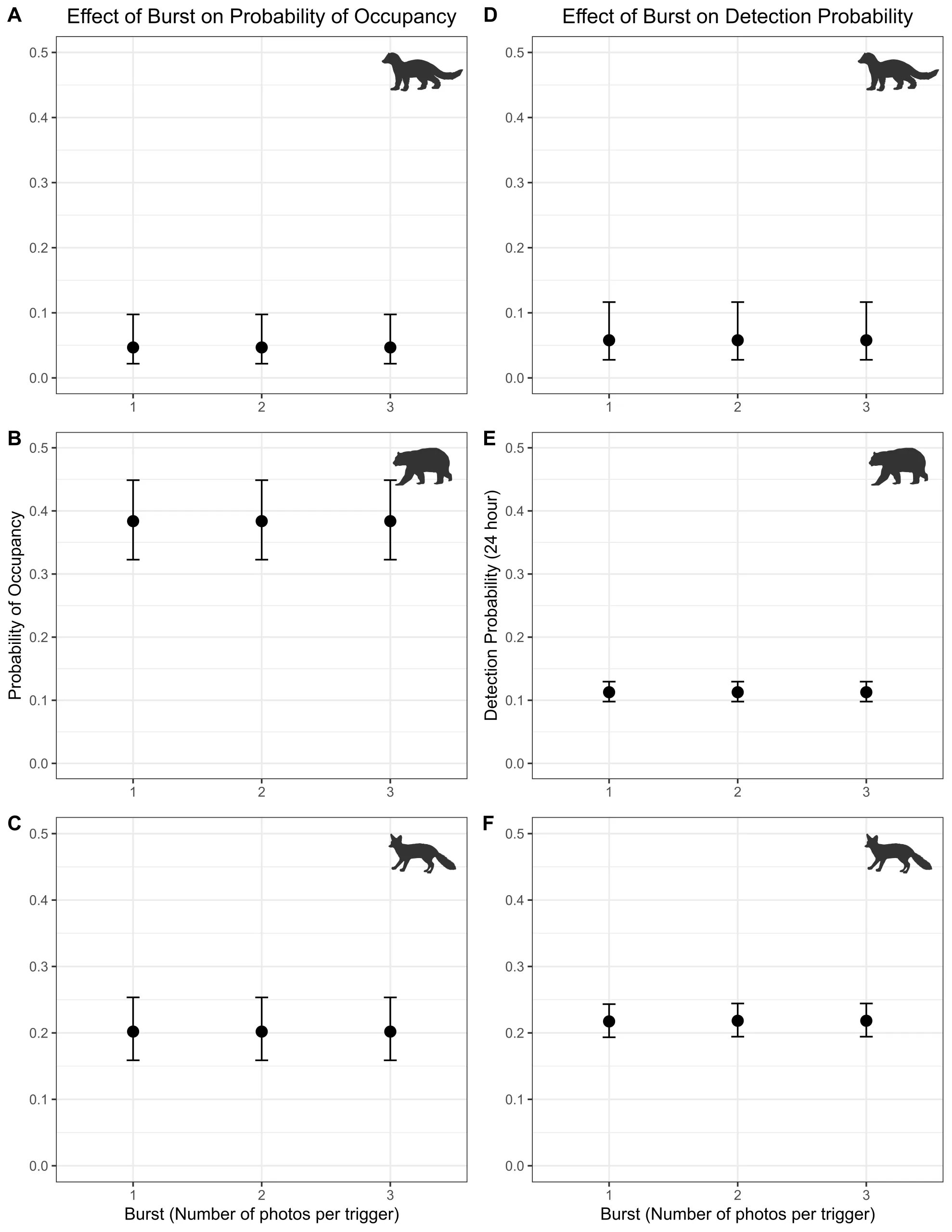
Figure 4. Plots of (A – C) occupancy and (D – F) detection probability for a single camera for each species by row for three different burst settings. Species results are organized by row with Row 1 = fisher, Row 2 = black bear, Row 3 = gray fox. Burst analysis only includes data from the 2016 Southwest Oregon study.
Discussion
The influence of internal camera settings that control the number of photos taken has received relatively little attention in the literature compared to other aspects of camera study design. Yet, these settings have major downstream implications for data management and analysis. Our results show that increasing delay period or reducing burst number decreased number of photos but did not meaningfully change occupancy or detection estimates for any species analyzed regardless of whether they were common or rare. However, changes to these settings did affect the photographic workload, with the dataset with shortest delay (5 sec) and highest burst (3) having >1,500% more photos than when that dataset was subset to the longest delay (300 sec) and lowest burst (1). These results indicate that, for occupancy analyses, setting too short a delay period or too high a burst number may only serve to increase photographic workload with little to no analytical benefit. These results concur with other studies that also found increasing delay periods had negligible effects on estimates of occupancy (Lepard et al., 2019), species richness (Mashintonio et al., 2022), or relative abundance indices (Sparkes et al., 2021).
Effects of additional photos on project workload and data storage needs can be significant. Extrapolating from the values observed in the camera data from this study, a project with 100 cameras running for 20 days could generate between 21,400 photographs (delay = 300s, burst = 1, cumulative photos/day = 214) to 324,500 photographs (delay = 5s, burst = 3, cumulative photos/day = 3,245). Assuming each photo is 5 MP, this difference corresponds to the need for ~32 GB of storage space for ~21,400 photos compared to ~487 GB for ~324,500 photos. To quantify this difference in terms of project workload, for example assuming a photo processing time of 1,000 photos/hour (processing rate varies widely by project and method used), 21,400 photos would take ~21 hours, versus ~325 hours to process 324,500 photos.
We found that increasing delay or decreasing burst settings had little to no effect on occupancy estimates whether the species was rare (fisher occupancy = 0.05) or common (black bear occupancy = 0.70). This occurs because occupancy analyses aggregate detections into a single presence/absence value per survey period, making one photo or multiple photos within that period equivalent for the encounter history. While we used 24-hour survey periods, many occupancy studies use longer multi-day periods corresponding to camera check intervals (e.g., Fisher et al. 2014: 7 days; Lukacs et al., 2020: 30 days). Longer survey periods inherently increase photo aggregation, and our 24-hour windows are shorter than the median 5-day detection windows commonly employed (Shannon et al., 2014, Burton et al., 2015). However, continuous camera trap monitoring often violates temporal independence assumptions, potentially underestimating occupancy probabilities and overestimating precision (Goldstein et al., 2024b). Given these aggregation effects, we expect delay and burst settings would have minimal impact on occupancy estimates using longer detection windows or larger camera arrays.
Our results pertain specifically to baited cameras used for occupancy analyses which are important factors to consider when interpreting our results. Using bait will increase time spent by an animal at a camera and can substantially increase the number of photos. For some species, bait and lure can significantly improve detection probability (du Preez et al., 2014, Lukacs et al., 2020) by increasing the likelihood an animal will encounter a camera, while for others, presence of bait can have little or no effect or even deter individuals (Avrin et al., 2020, 2021, Green et al., 2023), or can vary seasonally (Moriarty et al., 2018). If using unbaited cameras, a burst setting >1 and/or a short delay period may be important to adequately capture an identifiable image of an animal that might move quickly past the camera, particularly for highly mobile or hard to detect species. A similar study on how camera settings affect analyses using un-baited cameras would be a meaningful future endeavor.
There are numerous types of analyses that use camera trap data besides occupancy models, such as estimation of abundance (Gilbert et al., 2021), density (Rich et al., 2019, Green et al., 2020), species richness (Rich et al., 2017), or quantification of animal behavior (Caravaggi et al., 2017) including analyses of activity patterns (Rowcliffe et al., 2014) or diel niche (Mayer et al., 2023). Data needs and therefore optimal camera settings may differ depending on analysis type with some benefitting from a greater number or temporal frequency of photos (e.g., Leorna and Brinkman, 2024, Goldstein et al., 2024b), such as individual or sex identification (Karanth and Nichols, 1998, Rowland et al., 2020), or some activity pattern analyses (Peral et al., 2022). It is critical to carefully consider the study objective, analytical method, and species characteristics when choosing camera settings to avoid generating unnecessarily large photo datasets that only serve to increase the photo workload without significant analytical benefit. Our results indicate that for occupancy analyses for many species, multi-photo bursts and short delay periods are unnecessary and setting cameras to take single photos on longer delay periods yields comparable results while greatly reducing the number of photos and data management workload.
Acknowledgments
Thanks to S. Smyth, J. Buskirk, J. Ellison, and A. A. Orlando (Oregon study) and the numerous field technicians who contributed to both projects.
Author Contributions
Jody Tucker: Conceptualization, data curation, formal analysis, methodology, writing – original draft Jordan Heiman: Data curation, formal analysis, investigation, writing – original draft Jessie Golding: Conceptualization, data curation, formal analysis, methodology, writing – review and editing Brent Barry: Data curation, investigation, writing – review and editing Katie Moriarty: Data curation, investigation, writing – review and editing
Data Availability
All data and code can be found at the Repository https://doi.org/10.6084/m9.figshare.31795801.
Supplementary Information
Supplementary information can be found here.
Transparent Peer Review
Results from the Transparent Peer Review can be found here.
Recommended Citation
Tucker, J., J. Heiman, J. Golding, B. Barry, and K. Moriarty. 2026. How to avoid the camera trap: the effect of camera settings on occupancy analysis and photo data workload. Stacks Journal: 26003. https://doi.org/10.60102/stacks-26003
References
Ahumada, J. A., E. Fegraus, T. Birch, N. Flores, R. Kays, T. G. O’Brien, J. Palmer, S. Schuttler, J. Y. Zhao, W. Jetz, M. Kinnaird, S. Kulkarni, A. Lyet, D. Thau, M. Duong, R. Oliver, and A. Dancer. 2020. Wildlife Insights: A Platform to Maximize the Potential of Camera Trap and Other Passive Sensor Wildlife Data for the Planet. Environmental Conservation 47: 1–6. https://doi.org/10.1017/s0376892919000298.
Apps, P. J., and J. W. McNutt. 2018. How camera traps work and how to work them. African Journal of Ecology 56: 702–709. https://doi.org/10.1111/aje.12563.
Aubry, K. B., C. M. Raley, and P. G. Cunningham. 2018. Selection of rest structures and microsites by fishers in Oregon. The Journal of Wildlife Management 82: 1273–1284. https://doi.org/10.1002/jwmg.21479.
Avrin, A. C., C. E. Pekins, J. H. Sperry, and M. L. Allen. 2021. Evaluating the efficacy and decay of lures for improving carnivore detections with camera traps. Ecosphere 12: e03710. https://doi.org/10.1002/ecs2.3710.
Barry, B. R., K. Moriarty, D. Green, R. A. Hutchinson, and T. Levi. 2021. Integrating multi‐method surveys and recovery trajectories into occupancy models. Ecosphere 12: e03886. https://doi.org/10.1002/ecs2.3886.
Burnham, K. P., and D. R. Anderson. 2004. Multimodel inference: understanding AIC and BIC in model selection. Sociological Methods & Research 33: 261–304. https://doi.org/10.1177/0049124104268644.
Burton, A. C., E. Neilson, D. Moreira, A. Ladle, R. Steenweg, J. T. Fisher, E. Bayne, and S. Boutin. 2015. Wildlife camera trapping: a review and recommendations for linking surveys to ecological processes. Journal of Applied Ecology 52: 675–685. https://doi.org/10.1111/1365-2664.12432.
Caravaggi, A., P. B. Banks, A. C. Burton, C. M. Finlay, P. M. Haswell, M. W. Hayward, M. J. Rowcliffe, and M. D. Wood. 2017. A review of camera trapping for conservation behaviour research. Remote Sensing in Ecology and Conservation 3: 109–122. https://doi.org/10.1002/rse2.48.
Dart, M. M., L. B. Perkins, J. A. Jenks, G. Hatfield, and R. C. Lonsinger. 2022. The effect of scent lures on detection is not equitable among sympatric species. Wildlife Research 50: 190–200. https://doi.org/10.1071/wr22094.
Davis, C. L., L. N. Rich, Z. J. Farris, M. J. Kelly, M. S. Di Bitetti, Y. D. Blanco, S. Albanesi, M. S. Farhadinia, N. Gholikhani, and S. Hamel. 2018. Ecological correlates of the spatial co‐occurrence of sympatric mammalian carnivores worldwide. Ecology Letters 21: 1401–1412. https://doi.org/10.1111/ele.13124.
Delisle, Z. J., E. A. Flaherty, M. R. Nobbe, C. M. Wzientek, and R. K. Swihart. 2021. Next-generation camera trapping: systematic review of historic trends suggests keys to expanded research applications in ecology and conservation. Frontiers in Ecology and Evolution 9: 617996. https://doi.org/10.3389/fevo.2021.617996.
Du Preez, B. D., A. J. Loveridge, and D. W. Macdonald. 2014. To bait or not to bait: A comparison of camera-trapping methods for estimating leopard Panthera pardus density. Biological Conservation 176: 153–161. https://doi.org/10.1016/j.biocon.2014.05.021.
Evans, B. E., C. E. Mosby, and A. Mortelliti. 2019. Assessing arrays of multiple trail cameras to detect North American mammals. PLoS ONE 14: e0217543. https://doi.org/10.1371/journal.pone.0217543.
Fisher, J. T. 2025. Ecological insights from camera trapping span biological taxa, and the globe. Ecology and Evolution 15: e70947. https://doi.org/10.1002/ece3.70947.
Fisher, J. T., M. Wheatley, and D. Mackenzie. 2014. Spatial patterns of breeding success of grizzly bears derived from hierarchical multistate models. Conservation Biology 28: 1249–1259. https://doi.org/10.1111/cobi.12302.
Fiske, I., and R. Chandler. 2011. unmarked: An R Package for Fitting Hierarchical Models of Wildlife Occurrence and Abundance. Journal of Statistical Software 43: 1–23. https://doi.org/10.18637/jss.v043.i10.
Gilbert, N. A., J. D. J. Clare, J. L. Stenglein, and B. Zuckerberg. 2021. Abundance estimation of unmarked animals based on camera‐trap data. Conservation Biology 35: 88–100. https://doi.org/10.1111/cobi.13517.
Goldstein, B. R., A. G. Keller, K. L. Calhoun, K. J. Barker, F. Montealegre-Mora, M. W. Serota, A. Van Scoyoc, P. Parker-Shames, C. L. Andreozzi, and P. de Valpine. 2024a. How do ecologists estimate occupancy in practice? Ecography: e07402. https://doi.org/10.1111/ecog.07402.
Goldstein, B. R., A. J. Jensen, R. Kays, M. V. Cove, W. J. McShea, B. Rooney, E. M. Kierepka, and K. Pacifici. 2024b. Guidelines for estimating occupancy from autocorrelated camera trap detections. Methods in Ecology and Evolution 15:1177-1191. https://doi.org/10.1111/2041-210X.14359.
Green, A. M., M. W. Chynoweth, and Ç H. Şekercioğlu. 2020. Spatially explicit capture-recapture through camera trapping: a review of benchmark analyses for wildlife density estimation. Frontiers in Ecology and Evolution: 563477. https://doi.org/10.3389/fevo.2020.563477.
Green, D. S., M. E. Martin, S. M. Matthews, J. R. Akins, J. Carlson, P. Figura, B. E. Hatfield, J. D. Perrine, C. B. Quinn, and B. N. Sacks. 2023. A hierarchical modeling approach to predict the distribution and density of Sierra Nevada Red Fox (Vulpes vulpes necator). Journal of Mammalogy 104: 820-832. https://doi.org/10.1093/jmammal/gyad026.
Green, R. E., K. L. Purcell, C. M. Thompson, D. A. Kelt, and H. U. Wittmer. 2019. Microsites and structures used by fishers (Pekania pennanti) in the southern Sierra Nevada: a comparison of forest elements used for daily resting relative to reproduction. Forest Ecology and Management 440: 131-146. https://doi.org/10.1016/j.foreco.2019.02.042.
Hamel, S., S. T. Killengreen, J. Henden, N. E. Eide, L. Roed‐Eriksen, R. A. Ims, and N. G. Yoccoz. 2013. Towards good practice guidance in using camera‐traps in ecology: influence of sampling design on validity of ecological inferences. Methods in Ecology and Evolution 4: 105-113. https://doi.org/10.1111/j.2041-210x.2012.00262.x.
Hofmeester, T. R., N. H. Thorsen, J. P. Cromsigt, J. Kindberg, H. Andrén, J. D. C. Linnell, and J. Odden. 2021. Effects of camera-trap placement and number on detection of members of a mammalian assemblage. Ecosphere 12: e03662. https://doi.org/10.1002/ecs2.3662.
Iannarilli, F., J. Erb, T. W. Arnold, and J. R. Fieberg. 2021. Evaluating species-specific responses to camera-trap survey designs. Wildlife Biology 1: 1-12. https://doi.org/10.2981/wlb.00726.
Jacobs, C. E., and D. E. Ausband. 2018. An evaluation of camera trap performance – What are we missing and does deployment height matter? Remote Sensing in Ecology and Conservation 4: 352-360. https://doi.org/10.1002/rse2.81.
Jones, H. R. 2023. Habitat selection and habitat use of gray foxes (Urocyon cinereoargenteus) on trespass cannabis grows. MSc Thesis. California State Polytechnic University, Humboldt, Arcata, CA.
Karanth, K. U., and J. D. Nichols. 1998. Estimation of tiger densities in India using photographic captures and recaptures. Ecology 79: 2852-2862. https://doi.org/10.1890/0012-9658(1998)079[2852:EOTDII]2.0.CO;2.
Kays, R., B. S. Arbogast, M. Baker-Whatton, C. Beirne, H. M. Boone, M. Bowler, S. F. Burneo, M. V. Cove, P. Ding, S. Espinosa, A. L. S. Gonçalves, C. P. Hansen, P. A. Jansen, J. M. Kolowski, T. W. Knowles, M. G. M. Lima, J. Millspaugh, W. J. McShea, K. Pacifici, A. W. Parsons, B. S. Pease, F. Rovero, F. Santos, S. G. Schuttler, D. Sheil, X. Si, M. Snider, and W. R. Spironello. 2020. An empirical evaluation of camera trap study design: How many, how long and when? Methods in Ecology and Evolution 11: 700-713. https://doi.org/10.1111/2041-210X.13370.
Kellner, K. F., A. W. Parsons, R. Kays, J. J. Millspaugh, and C. T. Rota. 2022. A two-species occupancy model with a continuous-time detection process reveals spatial and temporal interactions. Journal of Agricultural, Biological and Environmental Statistics. 27: 321–338. https://doi.org/10.1007/s13253-021-00482-y.
Kristensen, T. V., and A. I. Kovach. 2018. Spatially explicit abundance estimation of a rare habitat specialist: implications for SECR study design. Ecosphere 9: e02217. https://doi.org/10.1002/ecs2.2217.
Lepard, C. C., R. J. Moll, J. D. Cepek, P. D. Lorch, P. M. Dennis, T. Robison, and R. A. Montgomery. 2019. The influence of the delay-period setting on camera-trap data storage, wildlife detections and occupancy models. Wildlife Research 46: 37–53. https://doi.org/10.1071/WR17181.
Linden, D. W., A. K. Fuller, J. A. Royle, and M. P. Hare. 2017. Examining the occupancy–density relationship for a low‐density carnivore. Journal of Applied Ecology 54: 2043–2052. https://doi.org/10.1111/1365-2664.12883.
Lonsinger, R. C., M. M. Dart, R. T. Larsen, and R. N. Knight. 2024. Efficacy of machine learning image classification for automated occupancy‐based monitoring. Remote Sensing in Ecology and Conservation 10: 56–71. https://doi.org/10.1002/rse2.356.
Lukacs, P. M., D. Evans Mack, R. Inman, J. A. Gude, J. S. Ivan, R. P. Lanka, J. C. Lewis, R. A. Long., R. Sallabanks, and Z. Walker. 2020. Wolverine occupancy, spatial distribution, and monitoring design. The Journal of Wildlife Management 84: 841–851. https://doi.org/10.1002/jwmg.21856.
Mackenzie, D. I., J. D. Nichols, G. B. Lachman, S. Droege, J. A. Royle, and C. A. Langtimm. 2002. Estimating site occupancy rates when detection probabilities are less than one. Ecology 83: 2248–2255. https://doi.org/10.1890/0012-9658(2002)083[2248:ESORWD]2.0.CO;2.
Manley, P. N., W. J. Zielinski, M. D. Schlesinger, and S. R. Mori. 2004. Evaluation of a multiple‐species approach to monitoring species at the ecoregional scale. Ecological Applications 14: 296–310. https://doi.org/10.1890/02-5249.
Mashintonio, A. F., G. M. Harris, D. R. Stewart, M. J. Butler, J. Sanderson, and G. Russell. 2022. Estimating species richness with camera traps: modeling the effects of delay period, deployment length, number of sites, and interference imagery. Wildlife Society Bulletin 46: e1357. https://doi.org/10.1002/wsb.1357.
Matthews, S.M., S. S. Greenleaf, H. M. Leithead, J. J. Beecham, and H. B. Quigley. 2003. Final Report: Bear Element Assessment Focused on Human-Bear Conflicts in Yosemite National Park Hornocker Wildlife, Institute Bozeman, Montana, USA.
Mayer, A. E., L. S. Ganoe, C. Brown, and B. D. Gerber. 2023. Diel activity structures the occurrence of a mammal community in a human‐dominated landscape. Ecology and Evolution 13: e10684. https://doi.org/10.1002/ece3.10684.
Meek, P. D., G. Ballard, and P. J. S. Fleming. 2015. The pitfalls of wildlife camera trapping as a survey tool in Australia. Australian Mammalogy 37: 13–22. https://doi.org/10.1071/AM14023.
Moriarty, K. M., M. A. Linnell, J. E. Thornton, and G. W. Watts. 2018. Seeking efficiency with carnivore survey methods: A case study with elusive martens. Wildlife Society Bulletin 42: 403–413. https://doi.org/10.1002/wsb.896.
Norouzzadeh, M. S., A. Nguyen, M. Kosmala, A. Swanson, M. S. Palmer, C. Packer, and J. Clune. 2018. Automatically identifying, counting, and describing wild animals in camera-trap images with deep learning. Proceedings of the National Academy of Sciences 115: E5716-E5725. https://doi.org/10.1073/pnas.1719367115.
O’Connell, A. F., J. D. Nichols, and K. U. Karanth. 2011. Camera traps in animal ecology: methods and analyses. New York: Springer. https://doi.org/10.1007/978-4-431-99495-4.
O’Connor, K. M., L. R. Nathan, M. R. Liberati, M. W. Tingley, J. C. Vokoun, and T. A. G. Rittenhouse. 2017. Camera trap arrays improve detection probability of wildlife: Investigating study design considerations using an empirical dataset. PLoS ONE 12:e0175684. https://doi.org/10.1371/journal.pone.0175684.
Oliver, R. Y., F. Iannarilli, J. Ahumada, E. Fegraus, N. Flores, R. Kays, T. Birch, A. Ranipeta, M. S. Rogan, and Y. V. Sica. 2023. Camera trapping expands the view into global biodiversity and its change. Philosophical Transactions of the Royal Society B 378: 1881. https://doi.org/10.1098/rstb.2022.0232.
Palencia, P., J. Vicente, R. C. Soriguer, and P. Acevedo. 2022. Towards a best-practices guide for camera trapping: assessing differences among camera trap models and settings under field conditions. Journal of Zoology 316: 197–208. https://doi.org/10.1111/jzo.12945.
Parker-Shames, P., B. R. Goldstein, and J. S. Brashares. 2024. Spatial and temporal activity of wildlife on and surrounding cannabis farms. The Stacks. https://doi.org/10.60102/stacks-24003.
Pease, B. S., C. K. Nielsen, and E. J. Holzmueller. 2016. Single-camera trap survey designs miss detections: impacts on estimates of occupancy and community metrics. PLoS ONE 11:e0166689. https://doi.org/10.1371/journal.pone.0166689.
Peral, C., M. Landman, and G. I. Kerley. 2022. The inappropriate use of time‐to‐independence biases estimates of activity patterns of free‐ranging mammals derived from camera traps. Ecology and Evolution 12: e9408. https://doi.org/10.1002/ece3.9408.
R Core Team. 2021. R: A language and environment for statistical computing. Version 4.5.0.
R Core Team. 2020. RStudio: Integrated Development for R. Version 2024.04.2
Rich, L. N., C. L. Davis, Z. J. Farris, D. A. W. Miller, J. M. Tucker, S. Hamel, M. S. Farhadinia, R. Steenweg, M. S. D. Bitetti, K. Thapa, M. D. Kane, S. S. Sunarto, N. P. Robinson, A. Paviolo, P. Cruz, Q. Martins, N. N. Gholikhani, A. Taktehrani, J. Whittington, F. A. Widodo, N. G. Yoccoz, C. Wultsch, B. J. Harmsen, and M. J. Kelly. 2017. Assessing global patterns in mammalian carnivore occupancy and richness by integrating local camera trap surveys. Global Ecology and Biogeography 26: 918–929. https://doi.org/10.1111/geb.12600.
Rich, L. N., D. A. W. Miller, D. J. Muñoz, H. S. Robinson, J. W. McNutt, and M. J. Kelly. 2019. Sampling design and analytical advances allow for simultaneous density estimation of seven sympatric carnivore species from camera trap data. Biological Conservation 233: 12–20. https://doi.org/10.1016/j.biocon.2019.02.018.
Rich, L. N., I. D. Medel, S. Bangen, G. M. Wengert, M. Toenies, J. M. Tucker, M. W. Gabriel, and C. L. Davis. 2023. Integrating existing data to assess the risk of an expanding land use change on mammals. Landscape Ecology 38: 3189–3204. https://doi.org/10.1007/s10980-023-01780-1.
Rowcliffe, J. M., R. Kays, B. Kranstauber, C. Carbone, and P. A. Jansen. 2014. Quantifying levels of animal activity using camera trap data. Methods in Ecology and Evolution 5: 1170–1179. https://doi.org/10.1111/2041-210X.12278.
Rowland, J., C. J. Hoskin, and S. Burnett. 2020. Camera traps are an effective method for identifying individuals and determining the sex of spotted-tailed quolls (Dasyurus maculatus gracilis). Australian Mammalogy 42: 349–356. https://doi.org/10.1071/AM19017.
Sparkes, J., P. J. S. Fleming, A. McSorley, and B. Mitchell. 2021. What are we missing? How the delay-period setting on camera traps affects mesopredator detection. Australian Mammalogy 43: 243–247. https://doi.org/10.1071/AM19068.
Steenweg, R., M. Hebblewhite, J. Whittington, and K. McKelvey. 2019. Species‐specific differences in detection and occupancy probabilities help drive ability to detect trends in occupancy. Ecosphere 10: e02639. https://doi.org/10.1002/ecs2.2639.
Steenweg, R., M. Hebblewhite, R. Kays, J. Ahumada, J. T. Fisher, C. Burton, S. E. Townsend, C. J. Carbone, M. Rowcliffe, J. Whittington, J. Brodie, J. A. Royle, A. Switalski, A. P. Clevenger, N. Heim, and L. N. Rich. 2017. Scaling-up camera traps: monitoring the planet’s biodiversity with networks of remote sensors. Frontiers in Ecology and the Environment 15: 26–34. https://doi.org/10.1002/fee.1448.
Steenweg, R., J. Whittington, M. Hebblewhite, A. Forshner, B. Johnston, D. Petersen, B. Shepherd, and P. M. Lukacs. 2016. Camera-based occupancy monitoring at large scales: Power to detect trends in grizzly bears across the Canadian Rockies. Biological Conservation 201: 192–200. https://doi.org/10.1016/j.biocon.2016.06.020.
Stewart, F. E., J. P. Volpe, and J. T. Fisher. 2019. The debate about bait: a red herring in wildlife research. The Journal of Wildlife Management 83: 985–992. https://doi.org/10.1002/jwmg.21657.
Tobler, M. W., S. E. Carrillo‐Percastegui, R. Leite Pitman, R. Mares, and G. Powell. 2008. An evaluation of camera traps for inventorying large‐and medium‐sized terrestrial rainforest mammals. Animal Conservation 11: 169–178. https://doi.org/10.1111/j.1469-1795.2008.00169.x.
Tucker, J. M., K. M. Moriarty, M. M. Ellis, and J. D. Golding. 2021. Effective sampling area is a major driver of power to detect long‐term trends in multispecies occupancy monitoring. Ecosphere 12: e03519. https://doi.org/10.1002/ecs2.3519.
Tuia, D., B. Kellenberger, S. Beery, B. R. Costelloe, S. Zuffi, B. Risse, A. Mathis, M. W. Mathis, F. Van Langevelde, and T. Burghardt. 2022. Perspectives in machine learning for wildlife conservation. Nature Communications 13: 1–15. https://doi.org/10.1038/s41467-022-27980-y.
US Fish and Wildlife Service. 2020. Endangered and threatened wildlife and plants; endangered species status for southern Sierra Nevada distinct population segment of fisher. Federal Register 85: 29532–29589.
Vélez, J., P. J. Castiblanco-Camacho, M. A. Tabak, C. Chalmers, P. Fergus, and J. Fieberg. 2022. Choosing an Appropriate Platform and Workflow for Processing Camera Trap Data using Artificial Intelligence. arXiv preprint arXiv:2202.02283. https://doi.org/10.1111/2041-210X.14044.
Zielinski, W. J., J. A. Baldwin, R. L. Truex, J. M. Tucker, and P. A. Flebbe. 2013. Estimating trend in occupancy for the southern Sierra fisher (Martes pennanti) population. Journal of Fish and Wildlife Management 4: 3–19. https://doi.org/10.3996/012012-JFWM-002.
Zielinski, W. J., J. M. Tucker, and K. M. Rennie. 2017. Niche overlap of competing carnivores across climatic gradients and the conservation implications of climate change at geographic range margins. Biological Conservation 209: 533–545. https://doi.org/10.1016/j.biocon.2017.03.016.
Open Access
Peer-Reviewed
Creative Commons


