Engineering orthogonal intensity and texture features for sample design, classification, regression, and clustering analyses using principal component analysis and convolution kernels

Introduction

Remotely sensed raster datasets of landscapes are commonly used as predictor variables (features) in many geospatial analyses. The information contained within these datasets span from cell values related to the earth’s surface (e.g., reflectance, temperature, and elevation) to patterns in cell values at coarser resolutions (texture) [1-5]. Both cell and texture values have been useful in sample design, classification, segmentation, and regression analyses [1-6] with a recent emphasis placed on texture and how texture can improve modeling results [1,3].

Within remote sensing, texture is quantified using convolution type analyses, which require specifying weights that are multiplied by cell values within a defined spatial window and summed together to attribute the center (focal) cell of a given window [5]. While many common image filters (kernels) have been defined and are used to enhance, blur, and identify edges and patterns in surrounding cell values [5], the number of kernels that can be defined are infinite, making it difficult to know which kernels best quantify texture. Moreover, many cell and texture values are highly correlated and covary across bands and neighboring cells within a neighborhood window, potentially making those features redundant and less desirable for modeling.

The classical approach to using texture in an analysis is to apply well known filters to input raster surfaces and use convolved outputs as features in a predictive model [7-9]. Alternatively, kernel weights can be optimally determined (learned) for a given task and applied to underlying remotely sensed data [3, 10, 11]. However, neither approach addresses covariance among band and neighboring cell values, which can have adverse effects on modeling and can substantially increase the total amount of processing.

One common approach to address covariance for continuous data is to project data along shared axes of covariance and create orthogonal features using a principal component analysis (PCA) [12]. For many remote sensing projects, PCAs have successfully been used to project multiband raster cell data onto orthogonal axes using component scores. Additionally, some of these same projects have successfully compressed the dimensionality of the data while retaining the majority of variation within the raster surface by selecting subsets of components that account for a known amount of variation in the data [13-16]. However, few remote sensing projects have addressed the issues of covariance in kernel cell values [9] and across image bands. Moreover, no studies have leveraged PCA component scores, derived from both band and neighboring cell values, to define kernel weights.

In this study we evaluate the use of a PCA to project multispectral imagery along orthogonal axes derived from both band and neighboring cell values. Our procedure automates the selection of optimal kernel weights for multidimensional convolution kernels based on principal component scores and the proportion of the variation (information in the data) explained by each component. To evaluate the utility of these components for modeling, we compare model fit and complexity for models derived from our components and models derived from common band and texture transformations. The spatial extent of our study includes portions of the Custer Gallatin National Forest located in southeastern Montana, USA (Figure 1).

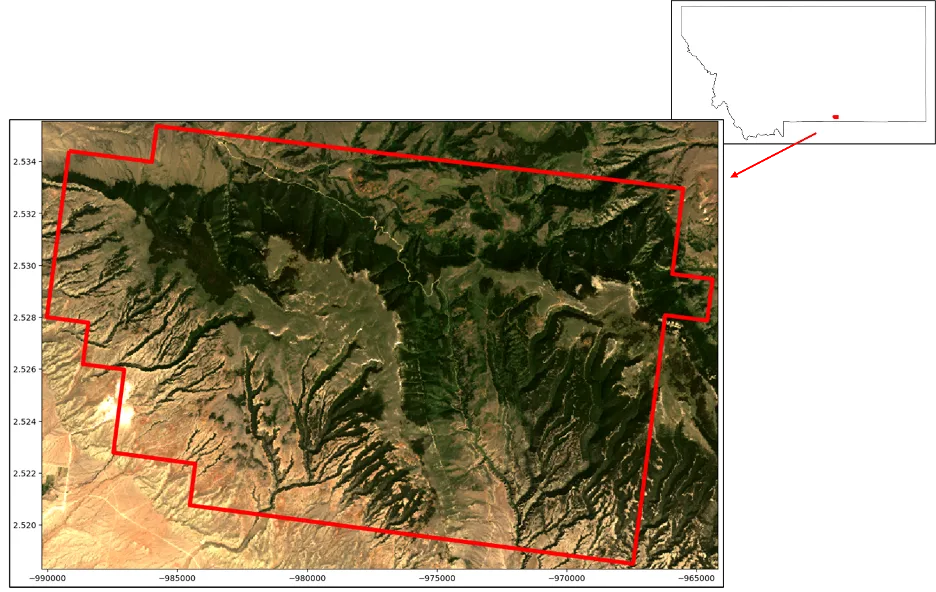
Figure 1. Study area location (top right) and boundary (bottom left).

Methods and Materials

Custer Gallatin national forest, located in southeastern Montana U.S., was chosen as our study site due to the variability of vegetative cover, species composition, topography, and the spatial transition from bare earth, grass, herbaceous vegetation, and forest cover types. To reduce download time associated with our example, we subset our study area to one part of the national forest’s multipart boundary polygon, covering approximately 31,600 ha. While our PCA convolution procedure can be applied to large raster surfaces, for brevity and ease of demonstration we used data collected for the subset of the Custer Gallatin national forest (Figure 1), using the steps described below.

1. 1. Download part of a Landsat scene [17] for the area around the Custer Gallatin Nation Forest (Figure 1) from Planetary Computer.

2. 2. Created a systematic random sample of locations using 10% of the cells within the Landsat image.

3. 3. Scaled sampled image band values by their standard deviation without centering [18].

4. 4. Extracted and flattened [19] surrounding neighbor cell values for a five by five window around each selected location.

5. 5. Performed a PCA [20].

6. 6. Extracted component eigen vector (score) values from the PCA for components that accounted for 95% of the variation in the data.

7. 7. Created component surfaces (CSs) by centering cell values and calculating the summed product of neighboring cell values and component scores.

8. 8. Scaled CS band cell values [21] to fall within 16 bits.

To perform these steps, we created a series of python functions that utilize Scikit Learn [22] and Raster Tools [23] application programming interface (API). Relevant functions and code used to perform these steps can be found within the “Estimating kernel weights using PCA and a defined analysis window” companion Jupyter notebook [24].

The Custer Gallatin national forest boundary was downloaded from OpenStreetMaps [25] using the osmnx package [26]. From the mulit-polygon returned for the geocode “Custer Gallatin National Forest, MT, USA”, we selected the first polygon greater than 31,000 ha to represent our study area. Landsat 8 imagery was downloaded using the extent of the selected Custer Gallatin national forests polygon and our get_stac_data function [24] that leveraged stackstac [27], pystac_client [28], and planetary-computer [29] packages. Scene selection dates ranged from 6/15/2016 to 6/30/2016 with an additional query of less than 10% cloud cover. In total, the downloaded Landsat 8 scene had seven spectral bands, 575 rows, and 868 columns. Functions used to download data can be found in the “Get Landsat 8 Imagery” section of the companion Jupyter notebook [24].

For our analysis, we created a PCA using approximately 10% of the cell locations systematically selected across image rows and columns. Randomization of the systematic selection process was achieved using random row and column starts [24]. Selected cell locations used for training represented the focal cell for each neighborhood window. Focal cell locations within each Landsat 8 image band were used to extract band cell values for a window size of five by five cells. Neighboring cell values within the corresponding image band and focal location were extracted using array slicing [30] and were further flattened to a one-dimensional array for downstream processing [24] (Figure 2).

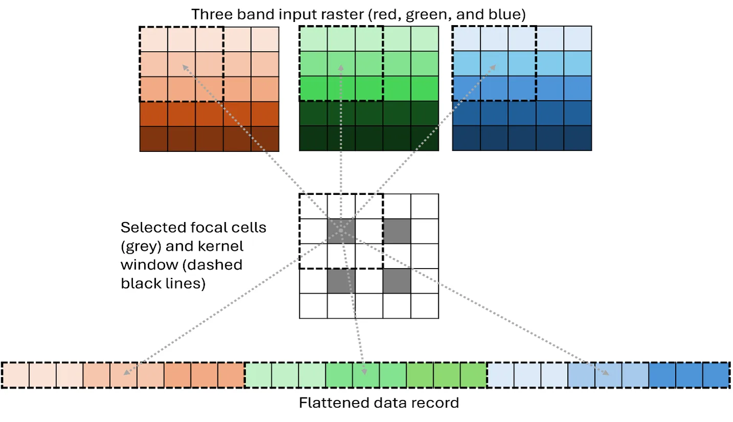
Figure 2. Depiction of a 3 by 3 kernel cell extraction and flattening method for the top left focal cell in a 5 by 5 cell image. Kernel cell values surrounding the top left focal cell are extracted row by column for each band within an image. Kernel cell values for the remaining focal cells are extracted in the same manner and are appended by row to the output dataset (4 rows, 27 columns).

Scaling [18, 21] and PCA [20] were performed using SciKit Learn’s preprocessing and decomposition modules. Standard Scaling was performed with centering omitted given that the PCA function centers all input features. Null values were excluded from the analysis to facilitate processing and image band masks [23] were applied to PCA convolved outputs to maintain consistency in null cell values. To implement the PCA convolution process, we leveraged Dask’s map_overlap function [31] and Numpy’s array arithmetic functions [32] within Raster Tools processing architecture [23]. Additionally, to decrease processing time, we used the Numba package for efficient looping [33]. Functions used to perform these steps can be found in the “Create convolution PCA model” section of the companion Jupyter notebook [24].

To evaluate the utility of convolution PCA for prediction purposes, we compared model fit and complexity for 100 random forest regression [34] and classification [35] trees models, derived from common remotely sensed texture metrics and convolution principal component values. For each of the 100 regression and classification models, 1120 training and 380 validation observations were randomly chosen from an initial 1500 locations selected at random across the study area. For consistency, the max_samples parameter for each model was set to 66% and the random_state parameter was set to zero. All other random forest modelling parameters were set to default values. To simplify the comparison between common texture and convolution PCA, we limited building texture to derivatives of the red and near infrared channels of the Landsat 8 imagery and limited the total number of observations used in developing and evaluating random forest models to 1500. Response surfaces used for comparisons included Percent Tree Canopy Cover [36] and National Land Cover Classification Dataset (NLCD) [37] for regression and classification trees, respectively. Texture metrics used in the comparison can be found in Table 1.

Results

Using our described approach, the first ten principal components accounted for 95% (summed eigen values proportion) of the variation within the Landsat 8 image (Figure 3). Component convolution kernel weights (eigen vectors) highlight the linear relationships among both Landsat image bands and neighboring window cell values. Comparing the magnitude and direction (positive or negative) of kernel weights provides insights into how band and neighboring cell values covary. For example, the first principal component accounted for approximately 75% of the variation in the data and can be described as a brightness component that averages cell values across neighboring cells and bands (Figure 4). The second principal component emphasized both intensity and texture across image bands and neighboring cells and can be generally described as a vegetative index that accounted for approximately 8% of the variation in the data. Additionally, the second principal component accentuates an inverse intensity relationship between infrared bands four and six along with aspects of texture in bands two and six [24]. Compared to the previous components, the third principal component accounted for approximately 4% of the variation in the data and can be described as a northwestern to southeastern texture gradient that clearly highlights differences in neighboring cell values along that gradient [24]. Each component’s eigen values and vectors can be interpreted in a similar manner to highlight laten aspects of the data that provide context regarding covariation in band and local neighborhood cell values.

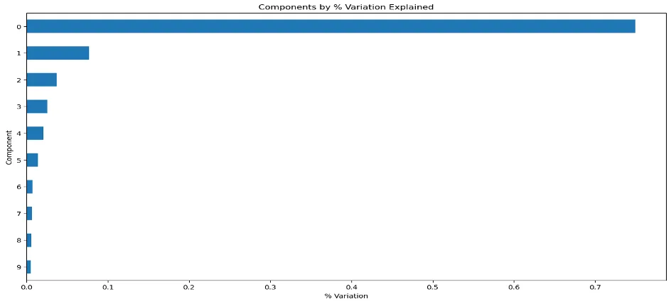
Figure 3. Proportion of variation explained in each principal component.

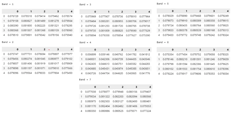
Figure 4. Five by five kernel weights, by band, for the first principal component.

For a random systematic sample of approximately 10% of the first 3 component values, it is apparent that there are unique groupings of information with varying trends in component space (Figure 5). Figure 5 displays component space from the perspective of the top, left, and right side of the data cube. While informative, static three dimensional renderings, such as Figure 5, only provide snapshots of the data. Additional information regarding how the data are projected as well as potential groupings become apparent when those data are rendered in a dynamic fashion, such as within the companion Jupyter notebook [24].

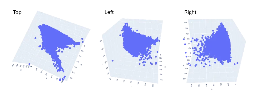
Figure 5. Three dimensional rendering of the first three principal components (0, 1, 2) rotated to highlight patterns in component space.

To transform our Landsat 8 image into ten CSs (Figure 6) required processing 70, 5 by 5 convolution kernels. Visually, each CS highlights a different aspect of the data within the original Landsat image and neighborhood window. Within each CS, linear combinations of both intensity and texture are highlighted to varying degrees and are projected such that each surface is orthogonal.

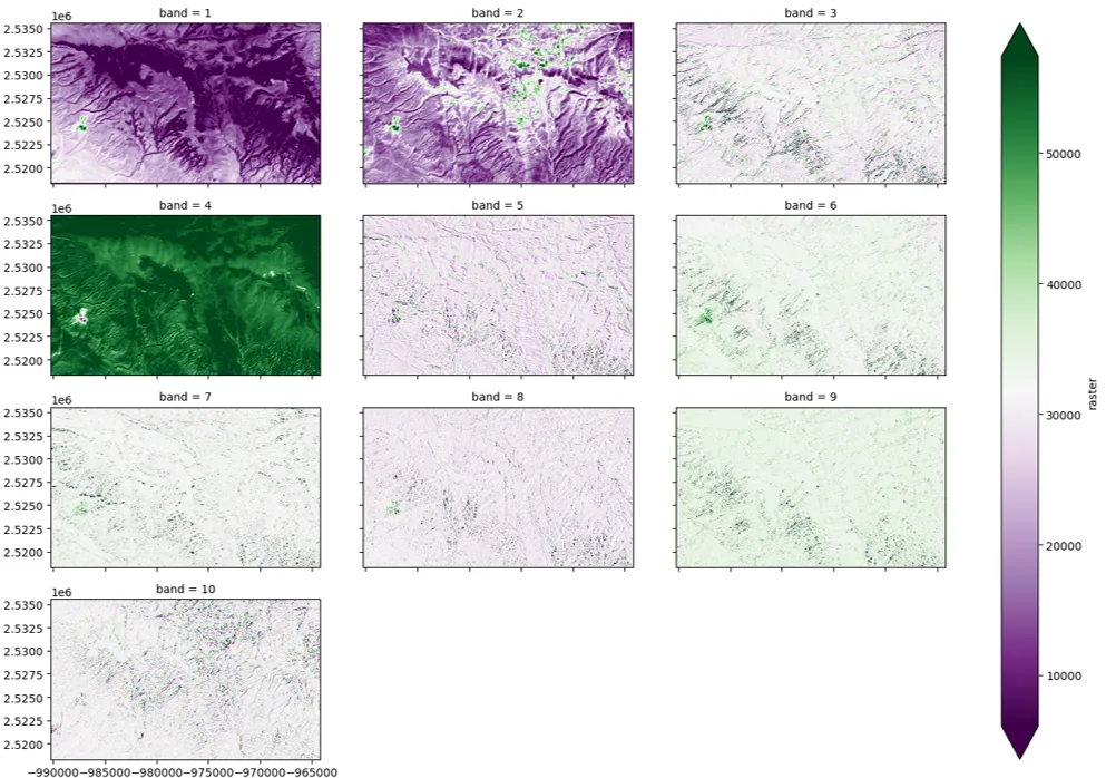
Figure 6. Ten orthogonal component surfaces (CSs) derived from the principal component analysis (PCA) convolution process.

While the kernel weights (Figure 4 and companion Jupyter notebook [24]) can be used to infer meaning for each component, it is often easier to look at the CSs to gain insights into the intensity and textural aspects of each component. For example, the first component (band 1) was generally described as a brightness component when interpreting the kernel weighs. Visually, this CS appears to support this description, highlighting cells and neighboring cell values that transition from purple to green as the intensity values transition from darker to lighter (Figure 6). Similarly, the second CS appears to highlight dark, forested, vegetation apparent in Figure 1, as intensity transitions from green to purple. Likewise, the third component (band 3) was described as a textural component given the kernel weights. This CS clearly highlights patches and edge as cell values transition from purple to green. Advantageously, each CS is orthogonal and clearly emphasizes varying combinations of intensity and spatial adjacency.

However, to explain the remaining 5% of the variation in the data, an additional 1155 convolution kernels would need to be processed. Using a threshold of 95% of the variation within the data substantially reduced the total amount of processing time needed to create CSs while simultaneously keeping the vast majority of information within the image. Moreover, implementing this processing within Raster Tools was easy and extremely efficient. Total processing time to transform the Landsat 8 image into 10 CSs took approximately 2 seconds using a conventional Intel CORE I7 processor with 8 cores and 16 gb of RAM.

Random Forest classification and regression models built using common texture metrics and our newly described convolution PCA method yielded similar results. The average overall validation accuracies of the 100 NLCD models was 79.5% (se = 0.018) and 79.8% (se = 0.021) for the common and PCA convolution texture-based models, respectively. Similarly, the root mean squared error derived from the validation datasets for the common and PCA texture-based models was 10.26 and 10.48, respectively (Table 2). While there were minor differences in modeled accuracy and error (Figure 7), the PCA convolution approach generally performed as well as using classical texture-based metrics using few predictors (Table 2).

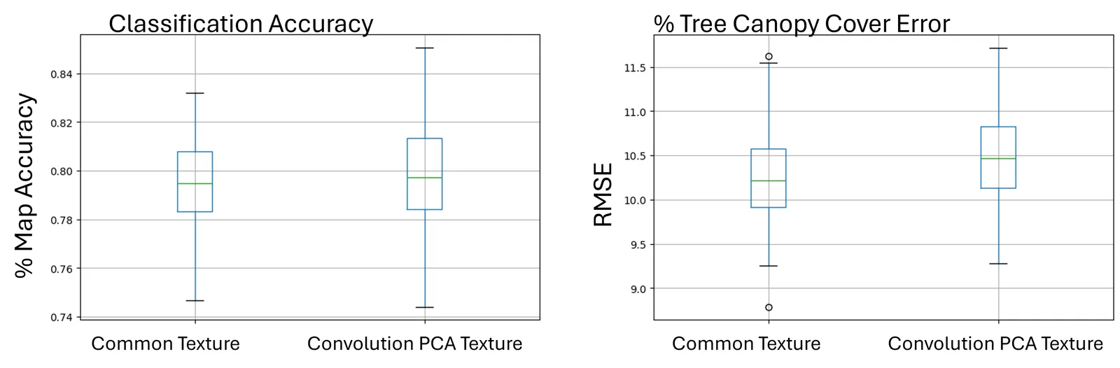
Figure 7. Boxplots of map accuracy and root mean squared error (RMSE) for 100 random forest models derived from common and PCA-based textures metrics

Discussion

We demonstrated how to use sampling, neighborhood windows, and PCA to project multi-band raster data into orthogonal component space (Figure 5) that highlights various aspects of the input data while simultaneously reducing the dimensionality of the data. The results of our analysis emphasize both intensity and textural aspects of the data within each principal component which can be viewed as a series of convolution kernel weights. While kernel cell weights provide unique insights into the linear relationships among image bands and neighbor cell values, when combined with Raster Tools processing architecture they can be used to produce CSs (Figure 6) that spatially emphasize independent intensity and textural aspects of the input data.

For example, the first CS in Figure 6 highlights an intensity change across spectral bands that emphasizes bright to dark cell values within the image. The kernel weights for the first component (Figure 4) verify this assertion with all positive values that generally share importance equally across all band kernels and cell values. When compared against the first CS (Figure 6), it is clear that the second CS emphasizes both an inverse relationship between infrared and other bands along with edges found in green and infrared bands. This appears to highlight a vegetation gradient transitioning from dense dark vegetation to non-vegetated areas (companion Jupyter Notebook [24]). CS three further highlights northwestern to southeastern linear edges that appear to correspond to vegetation changes in ridges and valleys in the imagery. Investigating the weights of each kernel for each component provides insights into the relative amounts of information (variation) within the data across both raster bands and neighboring cell space. However, the visual realization of the transformations (CSs) help to identify these relationships in geographic space, which highlights various patterns across the landscape and may provide insights into potential ecological processes.

Additionally, projecting band and neighboring cell values into orthogonal space provides a straightforward way to maintain as much information as possible within the data while simultaneously reducing the duplicated aspects of the data (Figure 3). In our example we ordered components based on the amount of variation explained in the data for that component and used a threshold of 95% of the total variation in the data to determine the number of CSs to create. Depending on the question at hand, analysts may want to select which components are relevant to the phenomenon of interest. Once decided and projected, CSs can be used as potential predictor variables in downstream analyses. Furthermore, when using deep learning techniques such as convolution neural networks (CNNs), kernel weights could be used as potential starting values to aid in solving for optimal kernel cell weights.

Compared to random forest models based on common texture metrics, models based on our described convolution principal components procedure, produced similar measures of accuracy and error. However, the convolution PCA approach required fewer predictors, removed issues of collinearity among cell values, and facilitated an automated approach to selecting features based on the proportion of variation explained in the data. Moreover, the PCA convolution technique learned optimal kernel weights, was simple and efficient to implement, simultaneously considered all cell combinations within a defined analysis window, and was easily interpreted numerically and visually (e.g., Figures 4 and 6). While this study fixed the analysis window to five by five cells, our approach can accommodate any window size and be used to combine texture metrics quantified at various spatial scales [24]. Given these beneficial traits, the convolution PCA approach to quantifying textures appears to be a good approach to integrating easily automated texture metrics into classification and regression models.

Although the objective of this study was to linearly project raster data across both image bands and neighboring cell values in a way that reduces the dimensionality of the data and determine a set of kernel weights used to produce CSs, our approach can also be used to optimize neighborhood window cell weights for regression and classification. The primary difference in this case would be regression or classification methodologies and response values would be used to optimally determine window cell weights. Moreover, CS values could also be inputs into deep learning methodologies. However, it is important to note CSs necessarily project the data across the entirety of the window cells. In the case of regression, classification, or deep learning, it may be advantageous to let the modeling approach learn the appropriate weights for each cell and potentially learn the optimal window size.

Conclusion

Our described approach provides an efficient and optimal solution that linearly describes unique intensity and textural aspects of the data across both raster bands and neighboring cell values, while simultaneously reducing the dimensionality of the data. The PCA convolution kernel approach to estimating kernel cell weights and convolving a raster dataset highlights various intensity and textural features in the dataset and mathematically determines kernel weights such that each band in the output convolved image is orthogonal. Moreover, our process is efficient and removes all redundant information across bands and within window cell values. Using this approach analysts can engineer orthogonal feature that can be used as predictor variables for modeling and aid in sample design.